Summary

• We present a method for performing circuit analysis on language models using "transcoders," an occasionally-discussed variant of SAEs that provide an interpretable approximation to MLP sublayers' computations. Transcoders are exciting because they allow us not only to interpret the output of MLP sublayers but also to decompose the MLPs themselves into interpretable computations. In contrast, SAEs only allow us to interpret the output of MLP sublayers and not how they were computed.
• We demonstrate that transcoders achieve similar performance to SAEs (when measured via fidelity/sparsity metrics) and that the features learned by transcoders are interpretable.
• One of the strong points of transcoders is that they decompose the function of an MLP layer into sparse, independently-varying, and meaningful units (like neurons were originally intended to be before superposition was discovered). This significantly simplifies circuit analysis, and so for the first time, we present a method for using transcoders in circuit analysis in this way.
• We performed a set of case studies on GPT2-small that demonstrate that transcoders can be used to decompose circuits into monosemantic, interpretable units of computation.
• We provide code for training/running/evaluating transcoders and performing circuit analysis with transcoders, and code for the aforementioned case studies carried out using these tools. We also provide a suite of 12 trained transcoders, one for each layer of GPT2-small. All of the code can be found at https://github.com/jacobdunefsky/transcoder_circuits, and the transcoders can be found at https://huggingface.co/pchlenski/gpt2-transcoders.

Work performed as a part of Neel Nanda's MATS 5.0 (Winter 2024) stream and MATS 5.1 extension. Jacob Dunefsky is currently receiving funding from the Long-Term Future Fund for this work.

Background and motivation

Mechanistic interpretability is fundamentally concerned with reverse-engineering models’ computations into human-understandable parts. Much early mechanistic interpretability work (e.g. indirect object identification) has dealt with decomposing model computations into circuits involving small numbers of model components like attention heads or MLP sublayers. 

But these component-level circuits operate at too coarse a granularity: due to the relatively small number of components in a model, each individual component will inevitably be important to all sorts of computations, oftentimes playing different roles. In other words, components are polysemantic. Therefore, if we want a more faithful and more detailed understanding of the model, we should aim to find fine-grained circuits that decompose the model’s computation onto the level of individual feature vectors.

As a hypothetical example of the utility that feature-level circuits might provide in the very near-term: if we have a feature vector that seems to induce gender bias in the model, then understanding which circuits this feature vector partakes in (including which earlier-layer features cause it to activate and which later-layer features it activates) would better allow us to understand the side-effects of debiasing methods. More ambitiously, we hope that similar reasoning might apply to a feature that would seem to mediate deception in a future unaligned AI: a fuller understanding of feature-level circuits could help us understand whether this deception feature actually is responsible for the entirety of deception in a model, or help us understand the extent to which alignment methods remove the harmful behavior.

Some of the earliest work on SAEs aimed to use them to find such feature-level circuits (e.g. Cunningham et al. 2023). But unfortunately, SAEs don’t play nice with circuit discovery methods. Although SAEs are intended to decompose an activation into an interpretable set of features, they don’t tell us how this activation is computed in the first place.^[1]

Now, techniques such as path patching or integrated gradients can be used to understand the effect that an earlier feature has on a later feature (Conmy et al. 2023; Marks et al. 2024) for a given input. While this is certainly useful, it doesn’t quite provide a mathematical description of the mechanisms underpinning circuits^[2], and is inherently dependent on the inputs used to analyze the model. If we want an interpretable mechanistic understanding, then something beyond SAEs is necessary.

Solution: transcoders

To address this, we utilize a tool that we call transcoders^[3]. Essentially, transcoders aim to learn a "sparsified" approximation of an MLP sublayer. SAEs attempt to represent activations as a sparse linear combination of feature vectors; importantly, they only operate on activations at a single point in the model. In contrast, transcoders operate on activations both before and after an MLP sublayer: they take as input the pre-MLP activations, and then aim to represent the post-MLP activations of that MLP sublayer as a sparse linear combination of feature vectors. In other words, transcoders learn to map MLP inputs to MLP outputs through the same kind of sparse, overparamaterized latent space used by SAEs to represent MLP activations.^[4]

The idea of transcoders has been discussed by Sam Marks and by Adly Templeton et al. Our contributions are to construct a family of transcoders on GPT-2 small, to provide a detailed analysis of the quality of transcoders (compared to SAEs) and their utility for circuit analysis, and to open source transcoders and code for using them.

Code can be found at https://github.com/jacobdunefsky/transcoder_circuits, and a set of trained transcoders for GPT2-small can be found at https://huggingface.co/pchlenski/gpt2-transcoders.

In the next two sections, we provide some evidence that transcoders display comparable performance to SAEs in both quantitative and qualitative metrics. Readers who are more interested in transcoders’ unique strengths beyond those of SAEs are encouraged to skip to the section “Circuit Analysis.”

Performance metrics

We begin by evaluating transcoders’ performance relative to SAEs. The standard metrics for evaluating performance (as seen e.g. here and here) are the following:

• We care about the interpretability of the transcoder/SAE. A proxy for this is the mean L0 of the feature activations returned by the SAE/transcoder – that is, the mean number of features simultaneously active on any given input.
• We care about the fidelity of the transcoder/SAE. This can be quantified by replacing the model’s MLP sublayer outputs with the output of the corresponding SAE/transcoder, and seeing how this affects the cross-entropy loss of the language model’s outputs.

There is a tradeoff between interpretability and fidelity: more-interpretable models are usually less faithful, and vice versa. This tradeoff is largely mediated by the hyperparameter λ1, which determines the importance of the sparsity penalty term in the SAE/transcoder loss. Thus, by training SAEs/transcoders with different λ1 values, we can visualize the Pareto frontier governing this tradeoff. If transcoders achieve a similar Pareto frontier to SAEs, then this might suggest their viability as a replacement for SAEs.

We trained eight different SAEs and transcoders on layer 8 of GPT2-small, varying the values of λ1 used to train them. (All SAEs and transcoders were trained at learning rate 4⋅10−4. Layer 8 was chosen largely heuristically – we figured that it’s late enough in the model that the features learned should be somewhat abstract and interesting, without being so late in the model that the features primarily correspond to “next-token-prediction” features.) The resulting Pareto frontiers are shown in the below graph:
 

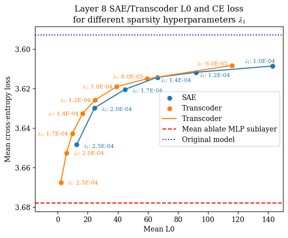
Importantly, it appears that the Pareto frontier for the loss-sparsity tradeoff is approximately the same for both SAEs and transcoders (in fact, transcoders seemed to do slightly better). This suggests that no additional cost is incurred by using transcoders over SAEs. But as we will see later, transcoders yield significant benefits over SAEs in circuit analysis. These results therefore suggest that going down the route of using transcoders instead of SAEs is eminently reasonable.

• (It was actually very surprising to us that transcoders achieved this parity with SAEs. Our initial intuition was that transcoders are trying to solve a more complicated optimization problem than SAEs, because they have to account for the MLP’s computation. As such, we were expecting transcoders to perform worse than SAEs, so these results came as a pleasant surprise that caused us to update in favor of the utility of transcoders.)

So far, our qualitative evaluation has addressed transcoders at individual layers in the model. But later on, we will want to simultaneously use transcoders at many different layers of the model. To evaluate the efficacy of transcoders in this setting, we took a set of transcoders that we trained on all layers of GPT2-small, and replaced all the MLP layers in the model with these transcoders. We then looked at the mean cross-entropy loss of the transcoder-replaced model, and found it to be 4.23 nats. When the layer 0 and layer 11 MLPs are left intact^[6], this drops down to 4.06 nats. For reference, recall that the original model’s cross-entropy loss (on the subset of OpenWebText that we used) was 3.59 nats. These results further suggest that transcoders achieve decent fidelity to the original model, even when all layers’ MLPs are simultaneously replaced with transcoders.

Qualitative interpretability analysis

Example transcoder features

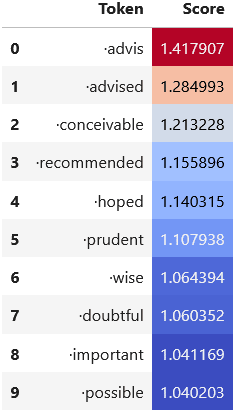
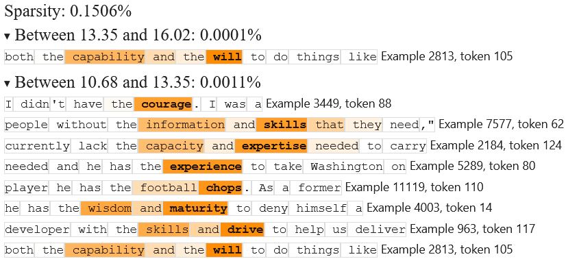
For a more qualitative perspective, here are a few cherry-picked examples of neat features that we found from the Layer 8 GPT2-small transcoder with λ1=8⋅10−5:

• Feature 31: positive qualities that someone might have
  
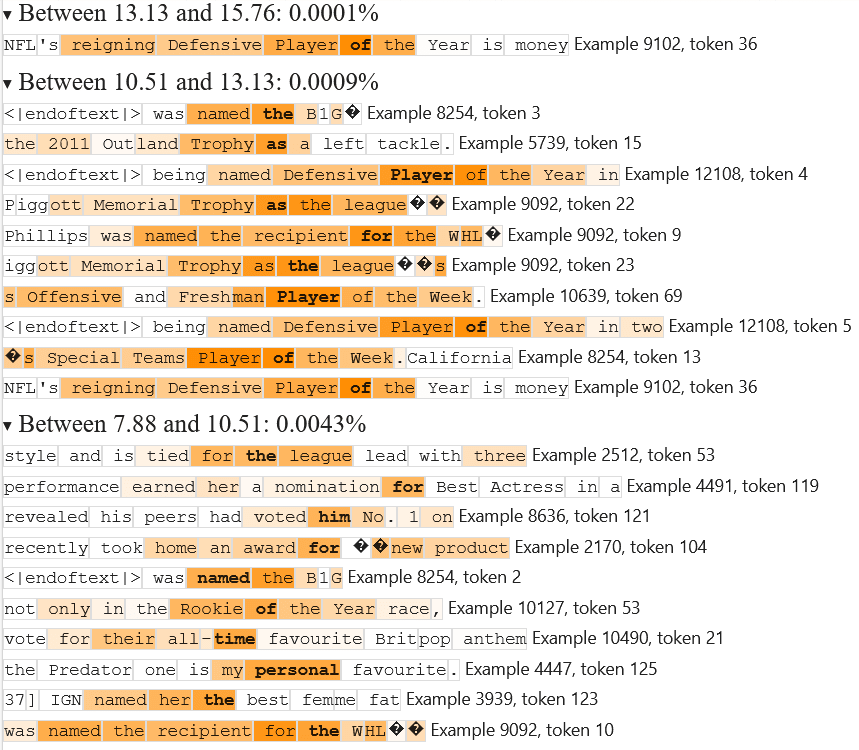
• Feature 15: sporting awards
  
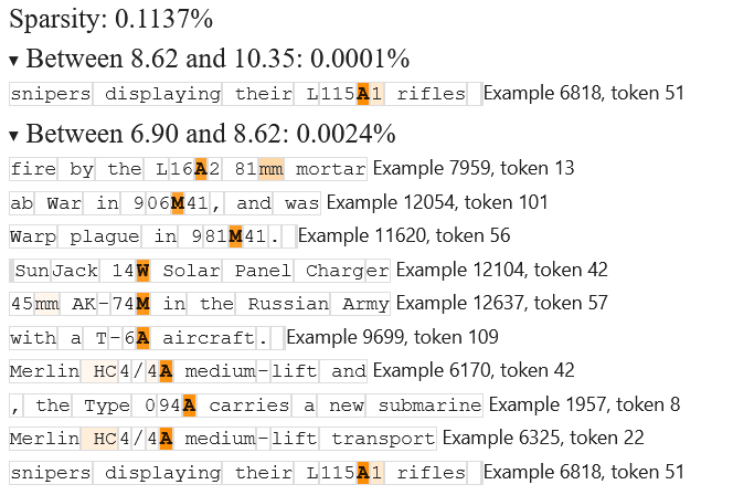
• Feature 89: letters in machine/weapon model names
  
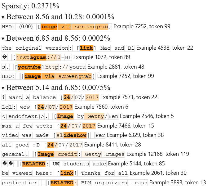
• Feature 6: text in square brackets
  

Broader interpretability survey

In order to get a further sense of how interpretable transcoder features are, we took the first 30 live features^[7] in this Layer 8 transcoder, looked at the dataset examples that cause them to fire the most, and attempted to find patterns in these top-activating examples.

We found that only one among the 30 features didn’t display an interpretable pattern^[8].

Among the remaining features, 5 were features that always seemed to fire on a single token, without any further interpretable patterns governing the context of when the feature fires.^[9] An additional 4 features fired on different forms of a single verb (e.g. fired on “fight”, “fights”, “fought”).

This meant that the remaining 20/30 features had complex, interpretable patterns. This further strengthened our optimism towards transcoders, although more rigorous analysis is of course necessary.

Circuit analysis

So far, our results have suggested that transcoders are equal to SAEs in both interpretability and fidelity. But now, we will investigate a feature that transcoders have that SAEs lack: we will see how they can be used to perform fine-grained circuit analysis that yields generalizing results, in a specific way that we will soon formally define.

Fundamentally, when we approach circuit analysis with transcoders, we are asking ourselves which earlier-layer transcoder features are most important for causing a later-layer feature to activate. There are two ways to answer this question. The first way is to look at input-independent information: information that tells us about the general behavior of the model across all inputs. The second way is to look at input-dependent information: information that tells us about which features are important on a given input.

Input-independent information: pullbacks and de-embeddings

The input-independent importance of an earlier-layer feature to a later-layer feature gives us a sense of the conditional effect that the earlier-layer feature firing has on the later-layer feature. It answers the following question: if the earlier-layer feature activates by a unit amount, then how much does this cause the later-layer feature to activate? Because this is conditional on the earlier-layer feature activating, it is not dependent on the specific activation of that feature on any given input.

This input-independent information can be obtained by taking the "pullback" of the later-layer feature vector by the earlier-layer transcoder decoder matrix. This can be computed as p=(Wdec)Tflater: multiply the later-layer feature vector flater by the transpose of the earlier-layer transcoder decoder matrix Wdec. Component i of the pullback p tells us that if earlier-layer feature i has activation k, then this will cause the later-layer feature’s activation to increase by kpi.^[10]

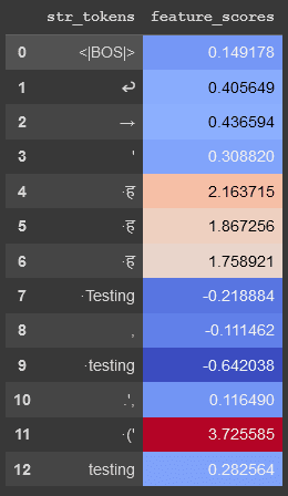
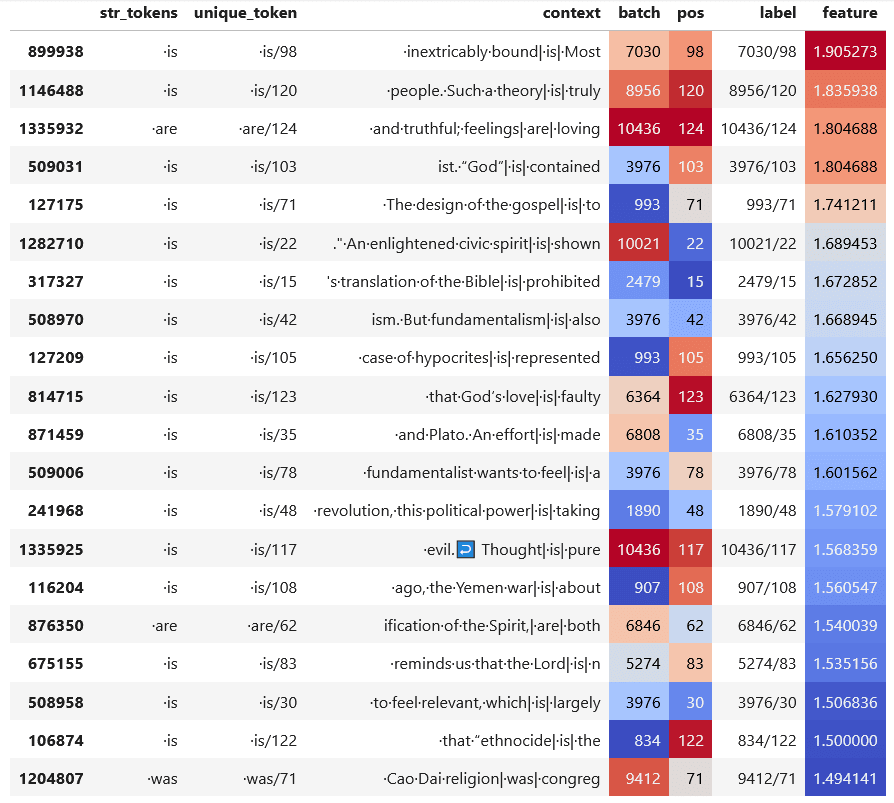
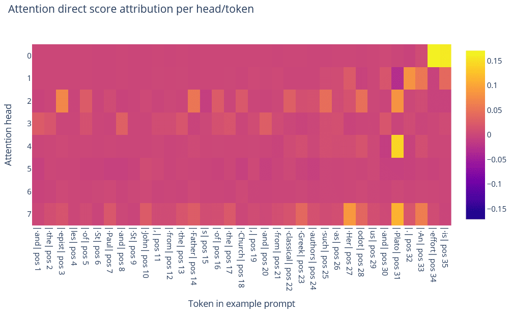
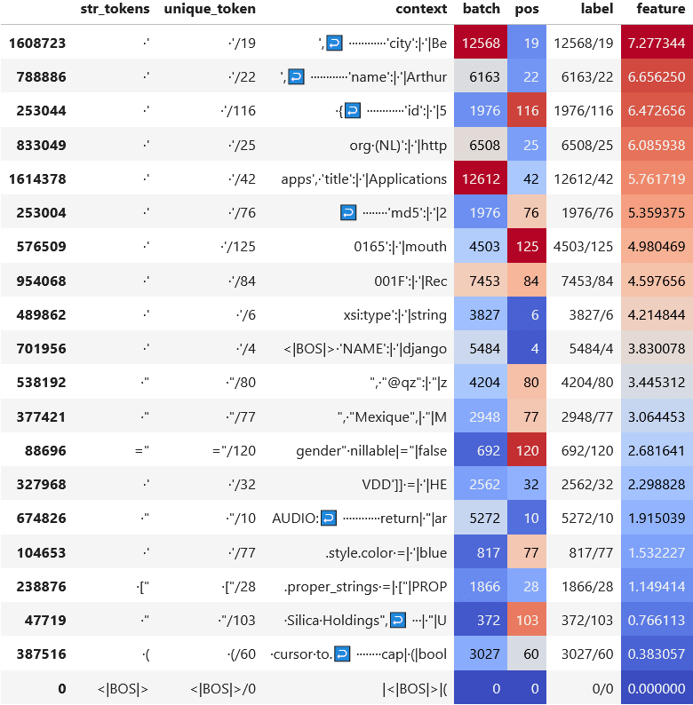
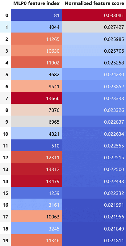
Here’s an example pullback that came up in one of our case studies:

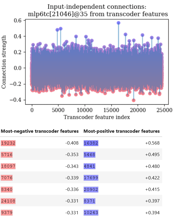
This shows how much each feature in a transcoder for layer 0 in GPT2-small will cause a certain layer 6 transcoder feature to activate. Notice how there are a few layer 0 features (such as feature 16382 and feature 5468) that have outsized influence on the layer 6 feature. In general, though, there are many layer 0 features that could affect the layer 6 feature.

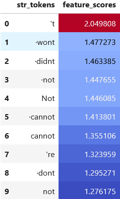
A special case of this “pullback” operation is the operation of taking a de-embedding of a feature vector. The de-embedding of a feature vector is the pullback of the feature vector by the model’s vocabulary embedding matrix. Importantly, the de-embedding tells us which tokens in the model’s vocabulary most cause the feature to activate.

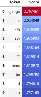
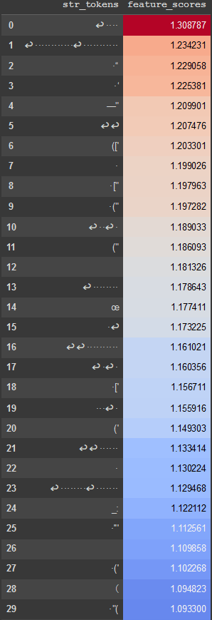
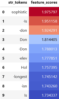
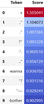
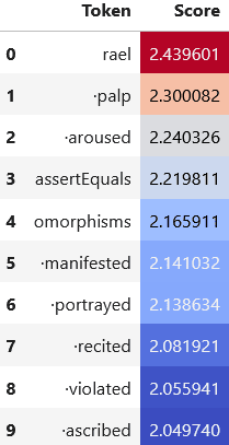
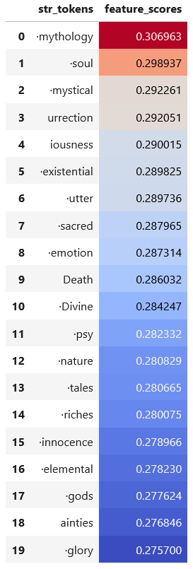
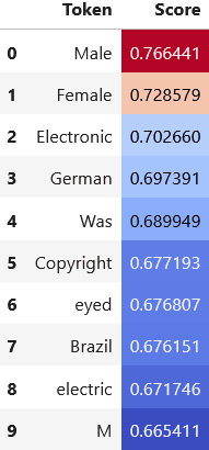
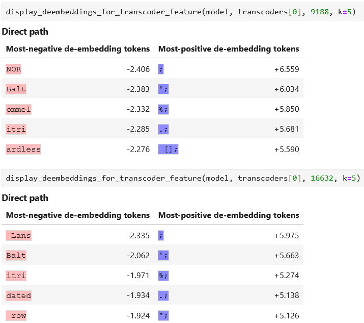
Here is an example de-embedding for a certain layer 0 transcoder feature:

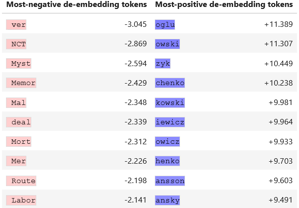
For this feature, the tokens in the model’s vocabulary that cause the feature to activate the most seem to be tokens from surnames – Polish surnames in particular.

Input-dependent information

There might be a large number of earlier-layer features that could cause a later-layer feature to activate. However, transcoder sparsity ensures only a small number of earlier-layer features will be active at any given time on any given input. Thus, only a small number will be responsible for the later-layer feature to activate.

The input-dependent influence q of features in an earlier-layer transcoder upon a later-layer feature vector f is given as follows: q=z(x)⊙p, where ⊙ denotes component-wise multiplication of vectors, z(x) is the vector of earlier-layer transcoder feature activations on input x, and p is the pullback of f with respect to the earlier-layer transcoder. Component i of the vector q thus tells you how much earlier-layer feature i contributes to feature f’s activation on the specific input x.

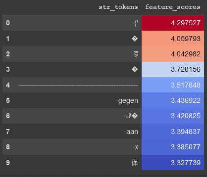
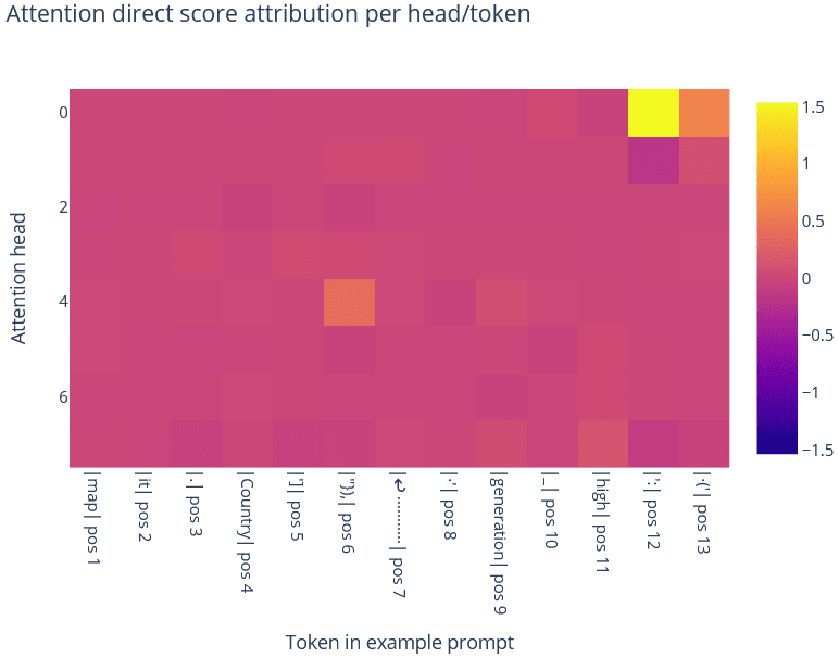
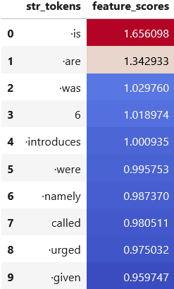
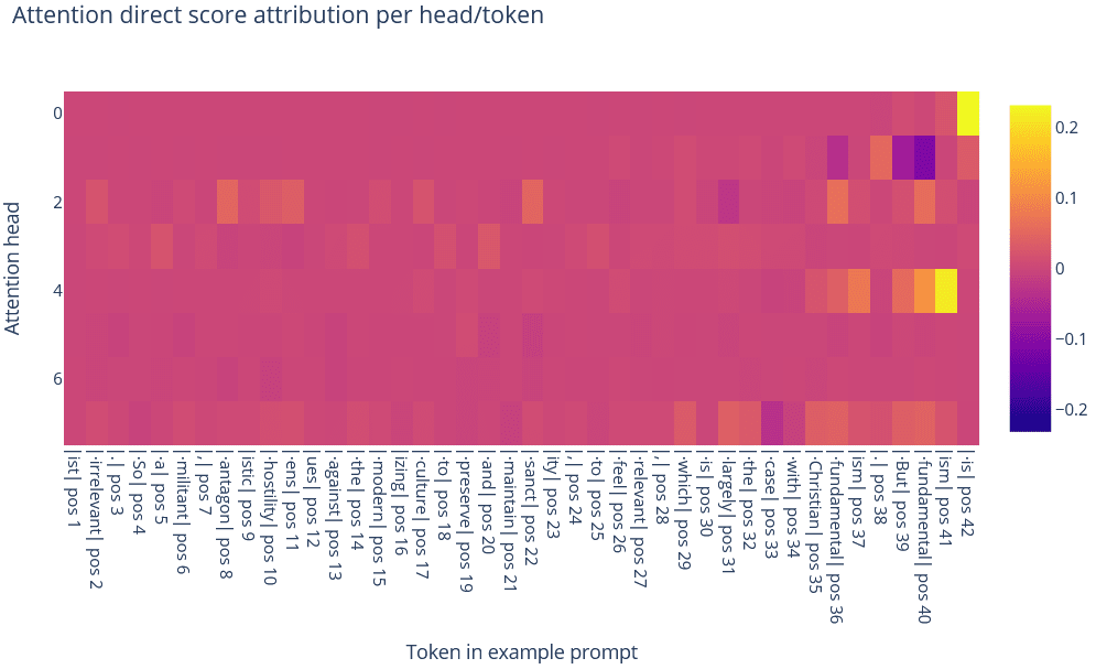
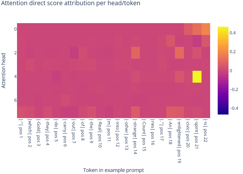
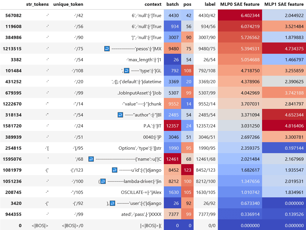
As an example, here’s a visualization of the input-dependent connections on a certain input for the same layer 6 transcoder feature whose pullback we previously visualized:

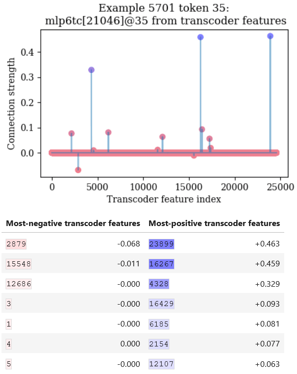
This means that on this specific input, layer 0 transcoder features 23899, 16267, and 4328 are most important for causing the layer 6 feature to activate. Notice how, in comparison to the input-independent feature connections, the input-dependent connections are far sparser.

• (Also, note that the top input-dependent features aren’t, in this case, the same as the top input-independent features from earlier. Remember: the top input-independent features are the ones that would influence the later-layer feature the most, assuming that they activate the same amount. But if those features are active less than others are, then those other features would display stronger input-dependent connections. That said, a brief experiment, which you can find in the appendix, suggests that input-independent pullbacks are a decent estimator of which input-dependent features will cause the later-layer feature to activate the most across a distribution of inputs.)

Importantly, this approach cleanly factorizes feature attribution into two parts: an input-independent part (the pullback) multiplied elementwise with an input-dependent part (the transcoder feature activations). Since both parts and their combination are individually interpretable, the entire feature attribution process is interpretable. This is what we formally mean when we say that transcoders make MLP computation interpretable in a generalizing way.

Obtaining circuits and graphs

We can use the above techniques to determine which earlier-layer transcoder features are important for causing a later-layer transcoder feature to activate. But then, once we have identified some earlier-layer feature i that we care about, then we can understand what causes feature i to activate by repeating this process, looking at the encoder vector for feature i in turn and seeing which earlier-layer features cause it to activate.

• This is something that you can do with transcoders that you can't do with SAEs. With an MLP-out SAE, even if we understand which MLP-out features cause a later-layer feature to activate, once we have an MLP-out feature that we want to investigate further, we're stuck: the MLP nonlinearity prevents us from simply repeating this process. In contrast, transcoders get around this problem by explicitly pairing a decoder feature vector after the MLP nonlinearity with an encoder feature before the nonlinearity.

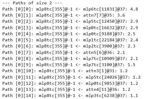
By iteratively applying these methods in this way, we can automatically construct a sparse computational graph that decomposes the model's computation on a given input into transcoder features at various layers and the connections between them. This is done via a greedy search algorithm, which is described in more detail in the appendix.

Brief discussion: why are transcoders better for circuit analysis?

As mentioned earlier, SAEs are primarily a tool for analyzing activations produced at various stages of a computation rather than the computation itself: you can use SAEs to understand what information is contained in the output of an MLP sublayer, but it’s much harder to use them to understand the mechanism by which this output is computed. Now, attribution techniques like path patching or integrated gradients can provide approximate answers to the question of which pre-MLP SAE features are most important for causing a certain post-MLP SAE feature to activate on a given input. But this local information doesn’t quite explain why those pre-MLP features are important, or how they are processed in order to yield the post-MLP output.

In contrast, a faithful transcoder makes the computation itself implemented by an MLP sublayer interpretable. After all, a transcoder emulates the computation of an MLP by calculating feature activations and then using them as the coefficients in a weighted sum of decoder vectors. These feature activations are both computationally simple (they’re calculated by taking dot products with encoder vectors, adding bias terms, and then taking a ReLU) and interpretable (as we saw earlier when we qualitatively assessed various features in our transcoder). This means that if we have a faithful transcoder for an MLP sublayer, then we can understand the computation of the MLP by simply looking at the interpretable feature activations of the transcoder.

As an analogy, let’s say that we have some complex compiled computer program that we want to understand (a la Chris Olah’s analogy). SAEs are analogous to a debugger that lets us set breakpoints at various locations in the program and read out variables. On the other hand, transcoders are analogous to a tool for replacing specific subroutines in this program with human-interpretable approximations.

Case study

In order to evaluate the utility of transcoders in performing circuit analysis, we performed a number of case studies, where we took a transcoder feature in Layer 8 in the model, and attempted to reverse-engineer it – that is, figure out mechanistically what causes it to activate. For the sake of brevity, we’ll only be presenting one of these case studies in this post, but you can find the code for the others at https://github.com/jacobdunefsky/transcoder_circuits. 

Introduction to blind case studies

The following case study is what we call a “blind case study.” The idea is this: we have some feature in some transcoder, and we want to interpret this transcoder feature without looking at the examples that cause it to activate. Our goal is to instead come to a hypothesis for when the feature activates by solely using the input-independent and input-dependent circuit analysis methods described above.

The reason why we do blind case studies is that we want to evaluate how well our circuit analysis methods can help us understand circuits beyond the current approach of looking for patterns in top activating examples for features. After all, we want to potentially be able to apply these methods to understanding complex circuits in state-of-the-art models where current approaches might fail. Furthermore, looking at top activating examples can cause confirmation bias in the reverse-engineering process that might lead us to overestimate the effectiveness and interpretability of the transcoder-based methods.

To avoid this, we have the following “rules of the game” for performing blind case studies:

• You are not allowed to look at the actual tokens in any prompts.
• However, you are allowed to perform input-dependent analysis on prompts as long as this analysis does not directly reveal the specific tokens in the prompt.
• This means that you are allowed to look at input-dependent connections between transcoder features, but not input-dependent connections from tokens to a given transcoder feature.
• Input-independent analyses are always allowed. Importantly, this means that de-embeddings of transcoder features are also always allowed. (And this in turn means that you can use de-embeddings to get some idea of the input prompt – albeit only to the extent that you can learn through these input-independent de-embeddings.)

Blind case study on layer 8 transcoder feature 355

For our case study, we decided to reverse-engineer feature 355 in our layer 8 transcoder on GPT2-small^[11]. This section provides a slightly-abridged account of the paths that we took in this case study; readers interested in all the details are encouraged to refer to the notebook case_study_citations.ipynb.

We began by getting a list of indices of the top-activating inputs in the dataset for feature 355. Importantly, we did not look at the actual tokens in these inputs, as doing so would violate the “blind case study” self-imposed constraint. The first input that we looked at was example 5701, token 37; the transcoder feature fires at strength 11.91 on this token in this input. Once we had this input, we ran our greedy algorithm to get the most important computational paths for causing this feature to fire. Doing so revealed contributions from the current token (token 37) as well as contributions from earlier tokens (like 35, 36, and 31).

First, we looked at the contributions from the current token. There were strong contributions from this token through layer 0 transcoder features 16632 and 9188. We looked at the input-independent de-embeddings of these layer 0 features, and found that these features primarily activate on semicolons. This indicates that the current token 37 contributes to the feature by virtue of being a semicolon.

Similarly, we saw that layer 6 transcoder feature 11831 contributes strongly. We looked at the input-independent connections from layer 0 transcoder features to this layer 6 feature, in order to see which layer 0 features cause the layer 6 feature to activate the most in general. Sure enough, the top features were 16632 and 9188 – the layer 0 semicolon features that we just saw.

The next step was to investigate computational paths that come from previous tokens in order to understand what in the context caused the layer 8 feature to activate. Looking at these contextual computational paths revealed that token 36 contributes to the layer 8 feature firing through layer 0 feature 13196, whose top de-embeddings are years like 1973, 1971, 1967, and 1966. Additionally, token 31 contributes to the layer 8 feature firing through layer 0 feature 10109, whose top de-embedding is an open parenthesis token.

Furthermore, the layer 6 feature 21046 was found to contribute at token 35. The top input-independent connections to this feature from layer 0 were the features 16382 and 5468. In turn, the top de-embeddings for the former feature were tokens associated with Polish last names (e.g. “kowski”, “chenko”, “owicz”) and the top de-embeddings for the latter feature were English surnames (e.g. “Burnett”, “Hawkins”, “Johnston”, “Brewer”, “Robertson”). This heavily suggested that layer 6 feature 21046 is a feature that fires upon surnames.

At this point, we had the following information:

• The current token (token 37) contributes to the extent that it is a semicolon.
• Token 31 contributes insofar as it is an open parenthesis.
• Various tokens up to token 35 contribute insofar as they form a last name.
• Token 36 contributes insofar as it is a year.

Putting this together, we formulated the following hypothesis: the layer 8 feature fires whenever it sees semicolons in parenthetical academic citations (e.g. the semicolon in a citation like “(Vaswani et al. 2017; Elhage et al. 2021)”.

We performed further investigation on another input and found a similar pattern (e.g. layer 6 feature 11831, which fired on a semicolon in the previous input; an open parenthesis feature; a year feature). Interestingly, we also found a slight contextual contribution from layer 0 feature 4205, whose de-embeddings include tokens like “Accessed”, “Retrieved”, “ournals” (presumably from “Journals”), “Neuroscience”, and “Springer” (a large academic publisher) – which further reinforces the academic context, supporting our hypothesis.

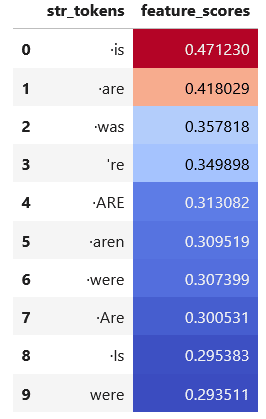
Evaluating our hypothesis

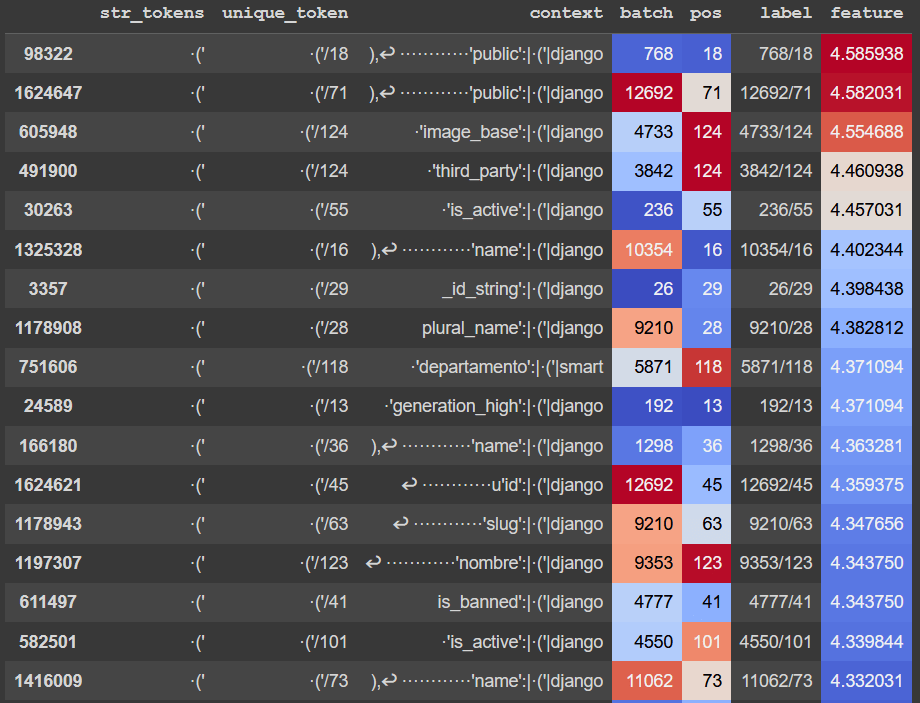
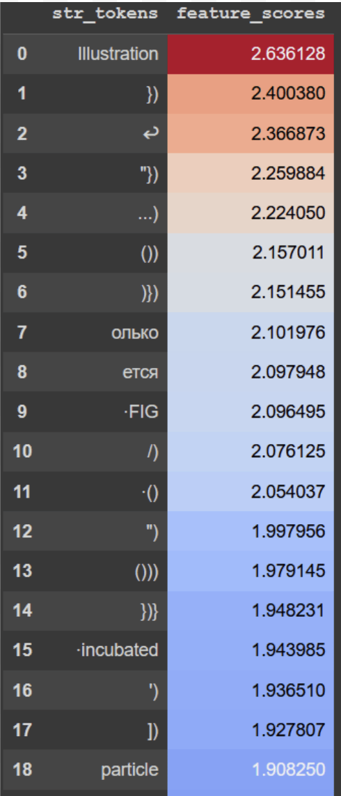
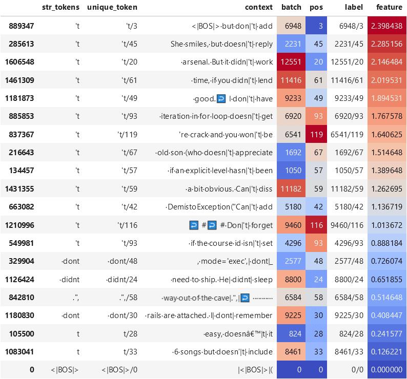
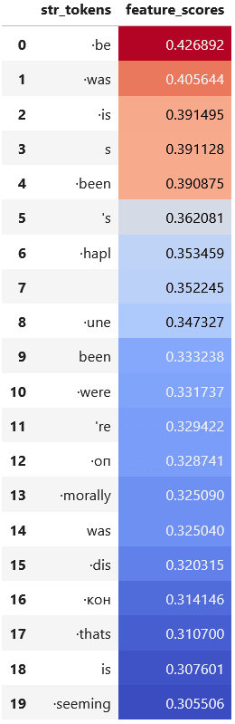
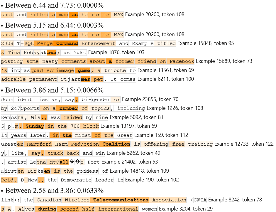
At this point, we decided to end the “blind” part of our blind case study and look at the feature’s top activating examples in order to evaluate how we did. Here are the results:
 

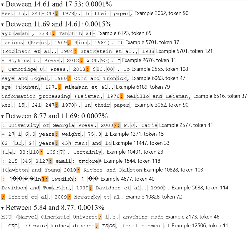
Yep – it turns out that the top examples are from semicolons in academic parenthetical citations! Interestingly, it seems that lower-activating examples also fire on semicolons in general parenthetical phrases. Perhaps a further investigation on lower-activating example inputs would have revealed this.

Code

As a part of this work, we’ve written quite a bit of code for training, evaluating, and performing circuit analysis with transcoders. A repository containing this code can be found at https://github.com/jacobdunefsky/transcoder_circuits/, and contains the following items:

• transcoder_training/, a fork of Joseph Bloom’s SAE training library with support for transcoders. In the main directory, train_transcoder.py provides an example script that can be adapted to train your own transcoders.
• transcoder_circuits/, a Python package that allows for the analysis of circuits using transcoders.
  • transcoder_circuits.circuit_analysis contains code for analyzing circuits, computational paths, and graphs.
  • transcoder_circuits.feature_dashboards contains code for producing “feature dashboards” for individual transcoder features within a Jupyter Notebook.
  • transcoder_circuits.replacement_ctx provides a context manager that automatically replaces MLP sublayers in a model with transcoders, which can then be used to evaluate transcoder performance.
• walkthrough.ipynb: a Jupyter Notebook providing an overview of how to use the various features of transcoder_circuits.
• case_study_citation.ipynb: a notebook providing the code underpinning the blind case study of an “academic parenthetical citation” feature presented in this post.
• case_study_caught.ipynb: a notebook providing the code underpinning a blind case study of a largely-single-token “caught” transcoder feature, not shown in this post. There is also a discussion of a situation where the greedy computational path algorithm fails to capture the full behavior of the model’s computation.
• case_study_local_context.ipynb: a notebook providing the code underpinning a blind case study of a “local-context” transcoder feature that fires on economic statistics, not shown in this post. In this blind case study, we failed to correctly hypothesize the behavior of the feature before looking at maximum activating examples, but we include it among our code in the interest of transparency.

Discussion

A key goal of SAEs is to find sparse, interpretable linear reconstructions of activations. We have shown that transcoders are comparable to SAEs in this regard: the Pareto frontier governing the tradeoff between fidelity and sparsity is extremely close to that of SAEs, and qualitative analyses of their features suggest comparable interpretability to SAEs. This is pleasantly surprising: even though transcoders compute feature coefficients from MLP inputs, they can still find sparse, interpretable reconstructions of the MLP output.

We think that transcoders are superior to SAEs because they enable circuit analysis through MLP nonlinearities despite superposition in MLP layers. In particular, transcoders decompose MLPs into a sparse set of computational units, where each computational unit consists of taking the dot product with an encoder vector, applying a bias and a ReLU, and then scaling a decoder vector by this amount. Each of these computations composes well with the rest of the circuit, and the features involved tend to be as interpretable as SAE features.

As for the limitations of transcoders, we like to classify them in three ways: (1) problems with transcoders that SAEs don’t have, (2) problems with SAEs that transcoders inherit, and (3) problems with circuit analysis that transcoders inherit:

1. So far, we’ve only identified one problem with transcoders that SAEs don’t have. This is that training transcoders requires processing both the pre- and post-MLP activations during training, as compared to a single set of activations for SAEs. 
2. We find transcoders to be approximately as unfaithful to the model’s computations as SAEs are (as measured by the cross-entropy loss), but we’re unsure whether they fail in the same ways or not. Also, the more fundamental question of whether SAEs/transcoders actually capture the ground-truth “features” present in the data – or whether such “ground-truth features” exist at all – remains unresolved.
3. Finally, our method for integrating transcoders into circuit analysis doesn’t further address the endemic problem of composing OV circuits and QK circuits in attention. Our code uses the typical workaround of computing attributions through attention by freezing QK scores and treating them as fixed constants.

At this point, we are very optimistic regarding the utility of transcoders. As such, we plan to continue investigating them, by pursuing directions including the following:

• Making comparisons between the features learned by transcoders vs. SAEs. Are there some types of features that transcoders regularly learn that SAEs fail to learn? What about vice versa?
• In this vein, are there any classes of computations that transcoders have a hard time learning? After all, we did encounter some transcoder inaccuracy; it would thus be interesting to determine if there are any patterns to where the inaccuracy shows up.
• When we scale up transcoders to larger models, does circuit analysis continue to work, or do things become a lot more dense and messy?

Of course, we also plan to perform more evaluations and analyses of the transcoders that we currently have. In the meantime, we encourage you to play around with the transcoders and circuit analysis code that we’ve released. Thank you for reading!

Author contribution statement

Jacob Dunefsky and Philippe Chlenski are both core contributors. Jacob worked out the math behind the circuit analysis methods, wrote the code, and carried out the case studies and experiments. Philippe trained the twelve GPT2-small transcoders, carried out hyperparameter sweeps, and participated in discussions on the circuit analysis methods. Neel supervised the project and came up with the initial idea to apply transcoders to reverse-engineer features.

Acknowledgements

We are grateful to Josh Batson, Tom Henighan, Arthur Conmy, and Tom Lieberum for helpful discussions. We are also grateful to Joseph Bloom for writing the wonderful SAE training library upon which we built our transcoder training code.

Appendix

For input-dependent feature connections, why pointwise-multiply the feature activation vector with the pullback vector?

Here's why this is the correct thing to do. Ignoring error in the transcoder's approximation of the MLP layer, the output of the earlier-layer MLP layer can be written as a sparse linear combination of transcoder features c1f1+...+ckfk, where the ci are the feature activation coefficients and the feature vectors fi are the columns of the transcoder decoder matrix Wdec. If the later-layer feature vector is flater, then the contribution of the earlier MLP to the activation of flater is given by c1fT1flater+...+ckfTkflater. Thus, the contribution of feature i is given by cifTiflater. But then this is just the i-th entry in the vector c⊙((Wdec)Tflater), which is the pointwise product of the pullback with the feature activations.

Note that the pullback is equivalent to the gradient of the later-layer feature vector with respect to the earlier-layer transcoder feature activations. Thus, the process of finding input-dependent feature connections is a case of the “input-times-gradient” method of calculating attributions that’s seen ample use in computer vision and early interpretability work. The difference is that now, we’re applying it to features rather than pixels.

Comparing input-independent pullbacks with mean input-dependent attributions

Input-independent pullbacks are an inexpensive way to understand the general behavior of connections between transcoder features in different layers. But how well do pullbacks predict the features with the highest input-dependent connections?

To investigate this, we performed the following experiment. We are given a later-layer transcoder feature and an earlier-layer transcoder. We can use the pullback to obtain a ranking of the most important earlier-layer features for the later-layer feature. Then, on a dataset of inputs, we calculate the mean input-dependent attribution of each earlier-layer feature for the later-layer feature over the dataset. We then look at the top k features according to pullbacks and according to mean input-dependent attributions, for different values of k. Then, to measure the degree of agreement between pullbacks and mean input-dependent attributions, for each value of k, we look at the proportion of features that are in both the set of top k pullback features and the set of top k mean input-dependent features.

We performed this experiment using two different (earlier_layer_transcoder, later_layer_feature) pairs, both of which pairs naturally came up in the course of our investigations.

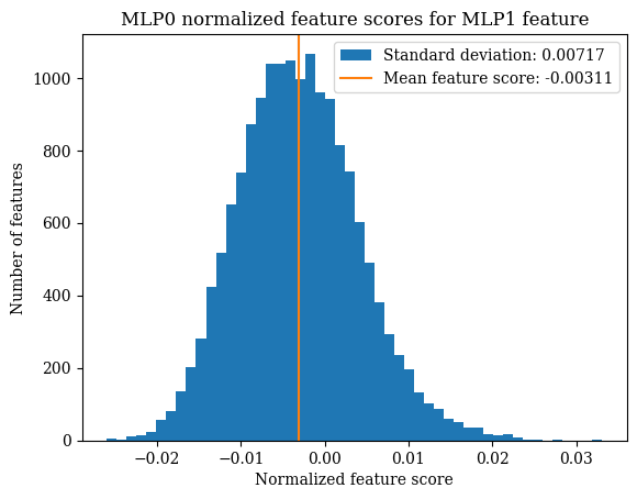
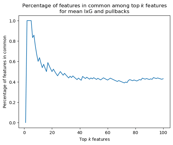
First, we looked at the connections from MLP0 transcoder features to MLP5 transcoder feature 12450.

• When k=10, then the proportion of features in both the top k pullback features and the top k mean input-dependent features is 60%.
• When k=20, then the proportion of common features is 50%.
• When k=50, then the proportion of common features is 44%.

The following graph shows the results for 1≤k≤100:

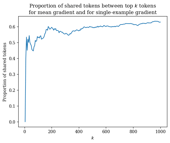
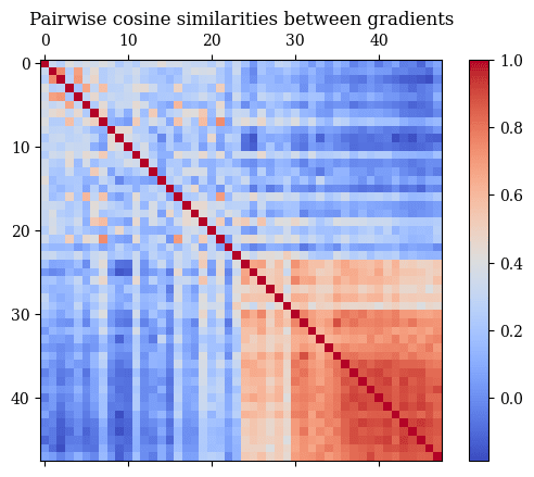
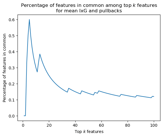
Then, we looked at the connections from MLP2 transcoder features to MLP8 transcoder feature 89.

• When k=10, then the proportion of features in both the top k pullback features and the top k mean input-dependent features is 30%.
• When k=20, then the proportion of common features is 25%.
• When k=50, then the proportion of common features is 14%.

The following graph shows the results for 1≤k≤100:

A more detailed description of the computational graph algorithm

At the end of the section on circuit analysis, we mention that these circuit analysis techniques can be used in an algorithm for constructing a sparse computational graph containing the transcoder features and connections between them with the greatest importance to a later-layer transcoder feature on a given input. The following is a description of this algorithm:

• Given: a feature vector, where we want to understand for a given input why this feature activates to the extent that it does on the input
• First, for each feature in each transcoder at each token position, use the input-dependent connections method to determine how important each transcoder feature is. Then, take the top k most important such features. We now have a set of k computational paths, each of length 2. Note that each node in every computational path now also has an "attribution" value denoting how important that node is to causing the original feature f to activate via this computational path.
• Now, for each path P among the k length-2 computational paths, use the input-dependent connections method in order to determine the top k most important earlier-layer transcoder features for P. The end result of this will be a set of k2 computational paths of length 3; filter out all but the k most important of these computational paths.
• Repeat this process until computational paths are as long as desired.
• Now, once we have a set of computational paths, they can be combined into a computational graph. The attribution value of a node in the computational graph is given by the sum of the attributions of the node in every computational path in which it appears. The attribution value of an edge in the computational graph is given by the sum of the attributions of the child node of that edge, in every computational path in which the edge appears.
• At the end, add error nodes to the graph (as done in Marks et al. 2024) to account for transcoder error, bias terms, and less-important paths that didn't make it into the computational graph. After doing this, the graph has the property that the attribution of each node is the sum of the attributions of its child nodes.

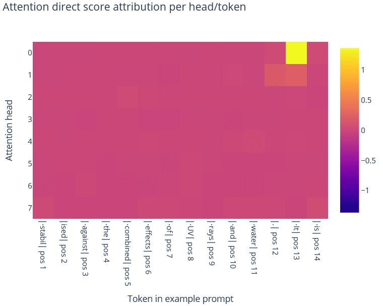
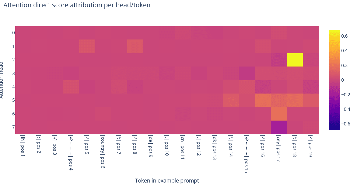
Note that the above description does not take into account attention heads. Attention heads are dealt with in the full algorithm as follows. Following the standard workaround, QK scores are treated as fixed constants. Then, the importance of an attention head for causing a feature vector to activate is computed by taking the dot product of the feature vector with the attention head’s output and weighting it by the attention score of the QK circuit (as is done in our previous work). The attention head is then associated with a feature vector of its own, which is given by the pullback of the later-layer feature by the OV matrix of the attention head.

The full algorithm also takes into account pre-MLP and pre-attention LayerNorms by treating them as constants by which the feature vectors are scaled, following the approach laid out in Neel Nanda’s blogpost on attribution patching).

Readers interested in the full details of the algorithm are encouraged to look at the code contained in transcoder_circuits/circuit_analysis.py.

Details on evaluating transcoders

In our evaluation of transcoders, we used 1,638,400 tokens taken from the OpenWebText dataset, which aims to replicate the proprietary training dataset used to train GPT2-small. These tokens were divided into prompts of 128 tokens each; our transcoders (and the SAEs that we compared them against) were also trained on 128-token-long prompts. Previous evaluations of SAEs suggest that evaluating these transcoders on longer prompts than those on which they were trained will likely yield worse results.

1. ^{^}

   In particular, if we want a method to understand how activations are computed, then it needs to account for MLP sublayers. SAEs could potentially help by disentangling these activations into sparse linear combinations of feature vectors. We thus might hope that the mappings between pre-MLP feature vectors and post-MLP features are likewise sparse, as this would give us a compact description of MLP computations. But SAE feature vectors are dense in the standard MLP basis; there are very few components close to zero. In situations such as dealing with OV circuits, this sort of basis-dependent density doesn’t matter, because you can just use standard linear algebra tools like taking dot products to obtain useful interpretations. But this isn’t possible with MLPs, because MLPs involve component-wise nonlinearities (e.g. GELU). Thus, looking at connections between SAE features means dealing with thousands of simultaneous, hard-to-interpret nonlinearities. As such, using SAEs alone won’t help us find a sparse mapping between pre-MLP and post-MLP features, so they don’t provide us with any more insight into MLP computations.

2. ^{^}

   When we refer to a “mathematical description of the mechanisms underpinning circuits,” we essentially mean a representation of the circuit in terms of a small number of linear-algebraic operations.

3. ^{^}

   Note that Sam Marks calls transcoders “input-output SAEs,” and the Anthropic team calls them “predicting future activations.” We use the term "transcoders," which we heard through the MATS grapevine, with ultimate provenance unknown.

4. ^{^}

   In math: an SAE has the architecture (ignoring bias terms) SAE(x)=WoutReLU(Winx), and is trained with the loss∥SAE(x)−x∥2+λ1∥ReLU(Winx)∥1, where λ1 is a hyperparameter and ∥⋅∥1 denotes the ℓ1 norm. In contrast, although a transcoder has the same architecture TC(x)=WoutReLU(Winx), it is trained with the loss ∥TC(x)−MLP(x)∥2+λ1∥ReLU(Winx)∥1, meaning that we look at the mean squared error between the transcoder’s output and the MLP’s output, rather than the transcoder’s output and its own input.

5. ^{^}

   Note that the mean ablation baseline doesn’t yield that much worse loss than the original unablated model. We hypothesize that this is due to the fact that GPT2-small was trained with dropout, meaning that “backup” circuits within the model can cause it to perform well even if an MLP sublayer is ablated.

6. ^{^}

   Empirically, we found that the layer 0 transcoder and layer 11 transcoder displayed higher MSE losses than the other layers’ transcoders. The layer 0 case might be due to the hypothesis that GPT2-small uses layer 0 MLPs as “extended token embeddings”. The layer 11 case might be caused by similar behavior on the unembedding side of things, but in this case, hypotheses non fingimus.

7. ^{^}

   A live feature is a feature that activates more frequently than once every ten thousand tokens.

8. ^{^}

   For reference, here is the feature dashboard for the lone uninterpretable feature:
   

   If you can make any sense of this pattern, then props to you.

9. ^{^}

   In contrast, here are some examples of single-token features with deeper contextual patterns. One such example is the word "general" as an adjective (e.g. the feature fires on “Last season, she was the general manager of the team” but not “He was a five-star general”). Another example is the word "with" after verbs/adjectives that regularly take "with" as a complement (e.g. the feature fires on “filled with joy” and “buzzing with activity”, but not “I ate with him yesterday”).

10. ^{^}

    The reason that the pullback has this property is that, as one can verify, the pullback is just the gradient of the later-layer feature activation with respect to the earlier-layer transcoder feature activations.

11. ^{^}

    As mentioned earlier, we chose to look at layer 8 because we figured that it would contain some interesting, relatively-abstract features. We chose to look at feature 355 because this was the 300th live feature in our transcoder (and we had already looked at the 100th and 200th live features in non-blind case studies).

Epistemic status: preliminary/exploratory.

Work performed as a part of Neel Nanda's MATS 5.0 (Winter 2023-2024) Research Sprint.

TL;DR: We develop a method for understanding how sparse autoencoder features in transformer models are computed from earlier components, by taking a local linear approximation to MLP sublayers. We study both how the feature is activated on specific inputs, and take steps towards finding input-independent explanations via examining model weights. We demonstrate this method with several deep-dive case studies to interpret the mechanisms used by simple transformers (GELU-1L and GELU-2L) to compute some specific features, and validate that it agrees with the results of causal methods.

Introduction

A core aim of mechanistic interpretability is tackling the curse of dimensionality, decomposing the high-dimensional activations and parameters of a neural network into individually understandable pieces. Sparse Autoencoders (SAEs) are a recent and exciting development that allows us to take high-dimensional activations (likely in superposition) and decompose them into meaningful directions in activation space that represent (mostly) independent concepts.

A major limitation of SAEs, when applied to MLP activations/outputs, is that it's difficult to study how a feature is computed from the output of earlier model components. With a meaningful neuron, we can look directly at its connections/virtual weights to earlier components -- e.g. a car neuron in a vision model being built from car window, car body, and car wheel neurons -- but SAE features are often dense in the neuron basis. This means that, naively, to understand how the feature is computed, we need to understand a complex non-linear function of the thousands of neuron activations. The curse of dimensionality remains!

In this post, we present a technique to explore how neuron-dense SAE features are computed from preceding model components. This approach involves taking the derivative of MLP sublayers in order to obtain a local linear approximation to the SAE feature -- a technique that has demonstrated some success in prior work such as attribution patching. Importantly, our method goes further and uses this linear approximation in conjunction with the model weights themselves to obtain a global picture of model behavior rather than one confined to a specific input example^[1]. The end result is an efficient way to obtain input-independent information about how the model computes SAE features.

We show this approach gives useful insights on a range of case studies, allowing us to reverse-engineer features back to the original token embeddings, and agrees with the results of causal interventions. We investigate how accurate and principled this approximation is. Though it's ultimately only an approximation, and may sometimes break down, we believe this is a useful tool that will allow a greater understanding of how SAE features are computed. 

Disclaimer: This is very preliminary work! We think these results are all rather exploratory; this post does not seek to make strong claims about how precisely we understand these SAE features and the mechanisms that compute them. But we hope that our results are interesting, that they may enable other people to build on them, and that they might help give better intuitions for thinking about SAEs. 

This post represents our output from a two week sprint as part of Neel Nanda's MATS 5.0 program, and we will keep building on it for the rest of the program. If you want to build on these ideas, please reach out! (Feel free to DM us on LessWrong, or if you'd prefer, send an email to [email protected])

Why is this important?

There are a number of reasons why we think this is an important problem to tackle:

• Reverse-engineering SAE features allows us to more effectively interpret them. In particular, doing so can reveal unexpected behavior that other methods might miss. For example, in one of our case studies, we find that a feature that initially seems to only activate on the token ('; after applying reverse-engineering, however, we find that the feature also activates on the token  ह, a Hindi character. Gaps in our understanding of SAE features limit their utility for predicting and analyzing unsafe or unwanted model behavior, so reverse-engineering is important in helping us identify these gaps.
• Reverse-engineering SAE features may reveal novel failure modes of a model. By understanding the algorithms that compute a given feature, we may better be able to understand what causes a model to exhibit undesired behavior. For instance, if we could find important downstream features in a model (such as whether a candidate would perform well in a job) and trace it back to protected characteristics of the input (such as race or gender), then we could use this to get a sense of the inherent bias in the model's computation.
• Reverse-engineering SAE features can help us better make theoretical claims about feature universality. For example, there is interest in understanding whether different models learn universal features. SAEs can be used to address this question by training SAEs on different models' activations and comparing the features that they learn (see the "universality" discussion from Anthropic's SAE paper). Because reverse-engineering reveals the mechanisms by which SAE features are computed, it could offer a complementary perspective for evaluating universality, by letting us test whether SAEs are useful for learning not just universal features but universal mechanisms. It may also help us catch illusory "universality", where features are superficially similar but are computed by different mechanisms and come apart in the right circumstances^[2].
• Reverse-engineering SAE features is useful for obtaining miscellaneous insights about the power and limitations of SAEs in general. For example, in one experiment on a 2-layer transformer, we use our method to express a layer-1 SAE feature in terms of layer-0 SAE features; we find that the connections between the layer-0 features and the layer-1 features are dense, indicating that SAEs as currently trained do not readily yield sparse information about how features at different layers of the same model relate to one another. This suggests that either internal model connections are just genuinely not sparse or that there are limitations to our SAE training methods, either of which is a useful insight! We expect there are many other insights about models and SAEs that we will only discover by doing deep dives into the internals of these models and how it all fits together.
• SAE features are an incomplete story without reverse-engineering. Just on a purely aesthetic level, we find it unsatisfying to be left in the dark regarding the computations that yield these features.

Overview

The rest of this post is organized into the following sections:

• We provide a high-level overview of the method that we use to carry out the reverse-engineering. We recommend reading this section because it provides useful context for understanding what is going on in our case studies. Readers interested in explicit mathematical details might be interested in reading the appendix section elaborating on this method.
• We present a number of case studies in which we reverse-engineer specific SAE features. This is the meat of our post, and where we expect most readers to get the most out of it (although we don't expect all readers to read through all the case studies). It is a long section, and we do go into very deep detail here,  but we think that it helps readers understand both what's how these features are computed and how the reverse-engineering process works in general. The following summary of our case studies might help you decide which ones you'd like to look at further:
  • A case study for a feature in GELU-1L that mostly fires on the token ('. 
    • In this case study, we use reverse-engineering to reveal that the seemingly monosemantic feature sometimes fires on unrelated tokens like  ह, a proof-of-concept for using this approach to construct adversarial prompts, and an example of how this approach can be used to understand unexpected behavior.
    • We also find that attention heads 0 and 3 contribute to the feature by firing on tokens indicating a code-related or list-related context.
  • A case study for a feature in GELU-1L that tends to fire on the bigram "it is" when preceded by punctuation. 
    • In this case study, we find that the direct path contributes to the feature by firing on the token  is as expected, and that attention head 0 fires on a preceding  It token. This allows us to understand a motif for computing bigram features.
  • A case study for a feature in GELU-1L that tends to fire on the token 't.
    • In this case study, we find that the direct path is very interpretable. Linearization suggests that attention is irrelevant, but the more reliable causal intervention of resample ablation suggests it does matter, suggesting that linearization was misleading here.
  • A case study for a feature in GELU-1L that tends to fire on the token  is in a theological/political context.
    • In this case study, we look at how the model computes a context-dependent feature largely via a single interpretable attention head.
  • A case study for a feature in GELU-2L that tends to fire on strings like {'name': '.
    • In this case study, we perform reverse-engineering in a two-layer model, including looking at the connection between layer 1 SAE features and layer 0 SAE features.
• We discuss MLP linearization in further depth, providing experimental results in order to begin to understand where this approach is valid and where it fails. This section can probably be skipped by most readers, although readers with a more theoretical interest in transformers or the validity of this method would likely get something out of reading it.
• We discuss our method’s benefits and drawbacks compared to causal methods like path patching. We recommend reading this brief section in order to understand where our method fits in with the broader landscape of mechanistic interpretability methods.
• We reflect on the method as a whole and what its strengths and limitations are. We recommend reading this brief section to calibrate your idea of where this method can be useful and what future directions might look like.

Our method

In this section, we present a high-level introduction to our method for reverse-engineering SAE features. For a more detailed explanation, interested readers should take a look at the "Appendix: Details on our method" section.

We apply and extend the method described in this post and in this paper for the purpose of reverse-engineering SAE features. We'll start by understanding how it works in a 1-layer transformer and then see how to scale this up.

Linearization: bringing an MLP feature into the residual stream

What goes into computing an SAE feature? Recall that a model's residual stream is the sum of the output of all previous model components. This means that if the feature is a linear function of the residual stream (i.e. the feature is computed by projecting the linear stream onto a given feature vector), then we could apply techniques such as direct feature attribution to understand how each model component contributes to the feature.

Unfortunately, for SAEs trained on MLP output activations, features "live" in MLP output space and not the residual stream. As such, before performing any further analysis, we have to pull back the SAE feature vector through the MLP, in order to obtain a feature vector in the residual stream corresponding to the original MLP output feature vector.

If MLPs were linear, then this could be done exactly -- but MLPs are not linear! They are complex nonlinear functions made up of many neurons, and most SAE features are dense, meaning that we would need to understand each neuron to understand the SAE feature. However, we can get a local linear approximation to an MLP by taking its gradient. This allows us to find a residual stream feature vector that approximately corresponds to the post-MLP feature vector. Concretely, we take the derivative of the SAE feature (pre-ReLU) with respect to the residual stream that is input to the MLP layer, on a specific token in a specific prompt.

Note that this is an activation-based technique rather than a weight-based technique; in other words, the obtained feature vector depends on the specific MLP activations, and different inputs result in different linearization feature vectors. We later investigate the consistency of these feature vectors and their accuracy.

Technical aside: freezing LayerNorm

Note that MLP sublayers (like all sublayers in a transformer) are preceded by LayerNorms, which consist of a linear transformation followed by a nonlinear normalization operation followed by a linear transformation. One can account for this nonlinearity by taking the gradient of the LayerNorm along with the MLP, but for reasons discussed later, this doesn't always yield good results. As such, it is sometimes necessary to freeze LayerNorms by ignoring the nonlinearity and only taking into account the linear transformations. (This means that when we apply a frozen LayerNorm to the residual stream, we still divide the residual stream by a value estimating the standard deviation of the residual stream -- but now, we treat this value as a constant, rather than as another function of the residual stream.)

A note on terminology: direct score attribution

Direct logit attribution is a well-known technique for understanding the contribution of model components to the logits of a model. Now that we have the residual stream feature vector, we can apply it to understand the contribution of model components to an SAE feature score as well. Since it doesn't make sense to talk about "logits" when looking at SAE feature scores, we instead refer to direct logit attribution on SAE features as direct score attribution throughout this post. The core idea is the same: decompose the residual stream into a sum of components, take the dot product of each component with the feature vector, and see which components are important.

The direct path and de-embedding

Now that we have a residual stream feature vector, we can use it to understand how the original token embedding contributes to the SAE feature activation. Following Elhage et al., we refer to this path from the original token embedding to the SAE feature as the direct path.

One way to interpret the direct path is by using a technique that we call de-embedding. The idea of de-embedding is to take the residual stream feature vector and take its dot product with each vector in the model's input embedding matrix; this yields a feature vector in the model's vocabulary space. Each token's coefficient in this vector provides an approximation of how much that token contributes to the SAE feature via the direct path. Importantly, one can look at the tokens whose coefficients in this vector are the highest in order to understand which tokens in the model's vocabulary are most important to the direct path.

Attention

Analyzing the OV circuit and the QK circuit

We can also use the residual stream feature vector to understand how different attention heads contribute to the SAE feature activation. Recall that an attention head's function can be decomposed into the QK circuit that computes attention scores and the OV circuit that transforms token information. Even though an attention head is a nonlinear function of the residual stream, if we look at the OV circuit in isolation, then the attention output is just the weighted sum of linear transformations for each attention head and each token.

As such, we can understand how the OV circuit for a given head contributes to the SAE feature by pulling the residual stream feature vector back through the OV matrix. Note that after doing this, we can then apply techniques like de-embedding to understand which tokens in the model's vocabulary contribute the most via that attention head's OV circuit to the SAE feature. In other words, we can determine which tokens, if attended to by that head, would most activate the feature. The QK circuit can then be analyzed separately by looking at which tokens have the highest QK scores with tokens that are important to the OV circuit.

Direct score attribution on (head, source token) pairs

One tool that we often use in our case studies is direct score attribution on individual (head, source token) pairs in attention. We can do this because the output of an attention head is a weighted sum of the contribution from each source token. This allows us to understand how much each source token contributes to the SAE feature through each attention head.

Multi-layer models

Computational paths

Things get somewhat more complicated in multi-layer transformers. This is because the set of possible computational paths from the input to the SAE feature increases (exponentially) with the number of layers. Different paths in a two-layer model might include:

• Token embeddings → MLP1 (the direct path)
• Token embeddings → MLP0 → attention 1 head 5 → MLP1
• Token embeddings → attention 0 head 3 → MLP0 → MLP1

However, the general principle is the same: keep pulling back the feature vector through each component in the path.

Note that some computational paths might involve multiple nonlinearities, such as two different MLP sublayers. In that case, we linearize through each nonlinearity separately. The more nonlinearities present in a computational path, the greater we expect the approximation error to be, but this can still yield useful results. Another option is to look at computational paths that, instead of going all the way back to the original token embedding, only go back to a previous layer's MLP. We will now see how this allows us to interpret paths to individual SAE features in such a previous MLP.

SAE virtual weights

One useful weights-based technique available in multi-layer models is the ability to write an SAE feature at a given layer in terms of a previous-layer SAE feature. We refer to this as looking at SAE virtual weights. To do this, take the residual stream feature vector for the later SAE feature, and pull it back through the decoder matrix of the previous-layer SAE. Just like de-embedding, as a result of this process, you obtain a vector that tells you how much each previous-layer SAE feature corresponds to the later SAE feature.

Other standard feature interpretation techniques

In addition to trying to reverse-engineer how the feature is computed, we follow Anthropic's approach to understanding these features by studying maximum/uniform activating examples and by studying the effect of each feature on the logits for each token in the model's vocabulary.

Maximum/uniform activating examples

One way to obtain an initial interpretation of an SAE feature is to look at which examples in a dataset activate that feature the most. However, following Anthropic's approach, it is also occasionally useful to sample examples across the full range of feature activation scores, in order to gain a broader understanding of what the feature represents. In this case, we find samples whose feature scores are uniformly spaced (to the best extent possible). For instance, if a certain feature is activated between 0.0 and 10.0 on a certain dataset, and we want to look at ten uniformly-spaced examples, then we would try and find an example with a feature score of 1.0, an example with a feature score of 2.0, etc.

Logit weights

Another approach used by Anthropic is to examine the effect that an SAE feature has on the logits of each token in the model's vocabulary. Intuitively, this gives us a sense of which tokens the model would expect to follow a token that highly activates the feature. The principle is similar to the logit lens: you do this by taking the decoder vector for the SAE feature and multiplying it by the model's unembedding matrix, and then looking at the tokens in the model's vocabulary that have the highest scores in the resulting vector. Sometimes, this can give us a good initial idea of how the model uses the feature, but this isn't always the case; as such, it can be useful to compare the understanding that we get by looking at logit weights with the understanding that we get by performing reverse-engineering.

Case studies

Experimental setup

The two models that we investigate are from Neel Nanda's ToyLM family, specifically the GELU-1L and GELU-2L models, which are (as the names suggest) a 1-layer and a 2-layer model respectively. The first four case studies are on GELU-1L, and the final one is on GELU-2L. These models were "trained on 22B tokens of data, 80% from C4 (web text) and 20% from Python code"; their model dimensionality dmodel is 512, their MLP dimensionality dmlp is 1,024, they have eight attention heads per attention sublayer, and their vocabulary contains 48,262 tokens.

When we use a dataset (e.g. to look at maximum activating examples), we use 1,638,400 tokens from c4-code-20k, which contains the same distribution of data as the datasets on which the models were trained. This corpus is divided into prompts of 128 tokens each.

The SAE that we investigate for GELU-1L is available as SAE #25 from this link, the final checkpoint for a single SAE training run, trained on GELU-1L activations by Neel Nanda. The SAEs that we investigate for GELU-2L are available as the SAEs prefixed by "gelu-2l" from this link. All SAEs have 16,384 features. The GELU-1L SAE is trained on the model's mlp_post activations (of dimension 1,024), while the GELU-2L SAEs are trained on the model's mlp_output activations (of dimension 512). You can find the code to use these SAEs here.

On the selection of features to study

The features addressed by the case studies were chosen in a relatively unprincipled manner, largely based off of what we thought would be interesting to study. Guiding our choice was a feature audit, which aimed to determine for all features the extent to which they exhibited context-dependence by calculating F1 scores for feature-token pairs. The reason that each feature was chosen is as follows:

• The (' feature was chosen because it was among the first high-frequency features (ordered by feature index, which has no intrinsic meaning).
• The it is feature was chosen because the feature audit suggested that it primarily activated on a single token, and only in very limited contexts, so we thought it would be cool to look into this further.
• The 't feature was chosen because the feature audit suggested that the feature highly activated on a single token, and on almost all occurrences of this token. As such, we wanted to investigate this seemingly context-independent feature.
• The "'is' in the context of theology/politics" feature was chosen largely at random.
• The GELU-2L feature was chosen because it was among the first high-frequency features.

Note that once we began a case study, we never abandoned it. As such, the results that you see account for all of the features that we investigated.

A  (' feature in GELU-1L

Maximum activating examples

Our first feature to investigate was feature 8 in the GELU-1L SAE. Looking at top activating examples suggested an immediate interpretation for this feature: a feature that primarily fires on the token  ('.

Logit weights

This SAE feature most strongly boosts the logits of the token django, which reflects what we see in the top activating examples. It also boosts the logits for other code-related tokens, like < and utf.

Direct path, and an unexpected finding

Now, we performed "de-embedding" in order to understand which tokens contribute the most to this feature through the direct path. Concretely:

• We differentiated through MLP0 with respect to this SAE feature's activation on a particular highly-activating example. This gave us a feature vector v of length dmodel in the residual stream.
• We multiplied this feature vector by the embedding matrix to see which tokens might activate it via the direct path, i.e. looked at the vector (WE)Tv of length dvocab. Naturally, we predict that  (' will score highly.

The results are given below:

The top token is, sure enough, the  (' token that we see in the top activating examples. But there are also some other unexpected tokens, such as the token  ह. This was surprising to us; in order to understand if this was a bug in our method, we ran the model on an adversarial prompt containing this token and recorded the raw feature activation (without taking into account the SAE bias or ReLU) for each token:

As we can see, the SAE feature actually does activate on this token, albeit not to the same extent as it does on the  (' token. This was surprising and exciting to us, because this was not apparent at all from the standard method of looking at top activating examples. We think this is an exciting proof of concept for our methods helping us construct adversarial examples for SAE features!^[3]

Attention

Performing direct score attribution on attention heads seemed to indicate that heads 0 and 3 were important. In the following example, we see that head 0 contributes to the feature through a ': token and the  (' token. Head 3 contributed to the feature through a closing parenthesis token "}),.

Looking at the OV circuit de-embedding for head 0^[4] indicated that the top tokens tended to include various opening string tokens like  ", ([', and the token  (' itself, but also various permutations of newlines followed by spaces. Interestingly, despite the high de-embedding score of the token  ', the direct score attribution example above indicates that this token didn't contribute much to the feature activation. This seems to be because head 0 did not attend as much to this token. Indeed, the pre-softmax attention score from the token  (' to the token  ' is 51.15, less than the pre-softmax attention score from the token  (' to the token ':, 63.86.

Among the top tokens in the OV circuit de-embedding for head 3 were many closing brace tokens, such as }), )}), and '). This suggests that head 3 contributes to the SAE feature via these closing brace tokens, in addition to initial whitespace tokens (as we see in the direct score attribution results). However, slightly complicating this picture is the fact that the top token in the de-embedding was the unrelated token  Illustration, which seemed to have no effect on feature scores when testing some initial adversarial prompts. Our later exploration of linearization suggests that the presence of tokens like this might be an artifact of linearly approximating the MLP.

Summary

Our reverse-engineering and de-embeddings, in conjunction with evidence obtained by looking at maximum activating examples, suggest that this feature has the following interpretation:

• The feature fires primarily on the token  (' in a code context -- in particular, in a context involving lists or tuples containing strings.
  • The direct path to the feature fires strongly on  ('.
  • Heads 0 and 3 establish a code context by firing on initial whitespace tokens.
  • Head 0 establishes a context involving lists and tuples containing strings by firing on tokens representing the beginning of such lists and tuples, such as the token  [". Head 3 establishes this context by firing on closing brace tokens such as }), )}), and ').
• But the feature also fires on the token  ह, albeit not as strongly!
  • This was an unexpected finding that came about after looking at the direct path de-embedding for this feature.

There still remain some unanswered questions, and some difficult-to-interpret results. In particular:

• The top token for the Head 3 OV de-embedding is  Illustration, which doesn't seem to contribute to the SAE feature in adversarial prompts. Is this a shortcoming of the method, or are there certain contexts in which this token does contribute to the feature?
• In this case study, we didn't look at QK circuits. Could this reveal more complex behavior, or maybe explain what's going on with the  Illustration token?

A feature for "[punctuation] it is" in GELU-1L

This is feature 4542 in the SAE that we're studying.

Maximum activating examples

This feature tended to maximally activate on the token  is when preceded by the token   it (or its capitalized variant), with the token  it often preceded by punctuation.

Logit weights

Looking at the logit weights for the SAE feature, the feature most boosts the logits for the tokens  advis,  advised,  conceivable,  recommended, and similar tokens -- all of which would tend to be used in impersonal constructions following "It is", such as "It is advisable that..."

Direct path

In the direct path de-embedding, when the pre-MLP LayerNorm is not taken into account, the top token for this feature is the token  is.

Note that the token  are, which has the second highest de-embedding score, slightly activates the feature when used in an adversarial prompt: the prompt . It are causes the feature to fire with score 0.151.

However, when linearizing the pre-MLP LayerNorm, the top tokens for this feature are rather more uninterpretable (although  Is is the second-highest-activating token). Potential theoretical underpinnings for why linearizing the pre-MLP LayerNorm might lead to these worse results are given in the section on linearization.

Attention

Performing direct score attribution on attention suggests that head 0, and to a lesser extent head 1, contribute to the feature by firing on tokens like "it". We also see that head 1 fires to some extent on punctuation tokens, although far less than the initial maximum activating examples might suggest.

Performing de-embedding on the OV circuit for head 0, surely enough, reveals that the top three tokens are variants of "it".

However, the de-embedding top tokens for head 1 are far more puzzling: all of the top twenty tokens are hard to interpret and seem to be unrelated to the feature, such as stitial,  undes, and  consc. Interestingly, it seems that these tokens can be used to construct adversarial prompts that activate the feature. For example, the prompt "then it is" causes the feature to fire with score 1.390, but the adversarial prompt "stitial it is" causes the feature to fire with score 1.521, and the adversarial prompt " undes it is" causes the feature to fire with score 1.626. (Note that the prompt ", it is" causes the feature to fire with score 1.733, higher than these adversarial prompts.)

Also surprising is that we don't see any punctuation tokens among the tokens with the top de-embedding scores for head 1 -- the token ., for instance, is only the 9097th-highest-scoring token. This is despite the fact that this token increases feature scores: the prompt . It is causes the feature to activate with score 1.903, whereas the prompt   It is only causes the feature to activate with score 1.820.

Summary

• The feature seems to activate on the token  is when preceded by tokens like  It,  it, and it.
  • The direct path de-embedding obtained without linearizing the pre-MLP LayerNorm reveals a high score for  is. However, when we linearize the pre-MLP LayerNorm, this yields many more uninterpretable tokens. This reflects certain behavior associated with linearizing LayerNorm that we discuss later.
• Head 0 contributes to the feature by firing on tokens like  it and  It. The top tokens in the de-embedding are, sure enough, It,  it, and  It.
• Direct score attribution suggests that head 1 contributes to the feature by slightly firing on punctuation tokens. However, this is not reflected in the de-embedding for head 1, which is wholly uninterpretable. A more in-depth investigation might clarify what is happening with punctuation.

A 't feature in GELU-1L

This is feature number 10996 in the SAE that we're studying.

Uniform activating examples

Looking at examples on which this feature activates, it seems that this feature primarily activates on the token 't at the end of words like "doesn't", "don't", "won't", and the like^[5]. At lower levels of activation, this feature also fires on misspellings like "dont" and "didnt".

Logit weights

This feature most strongly boosts the logits for the token s and tokens consisting of punctuation followed by a quotation mark. This isn't reflected in the uniform activating examples, suggesting that looking at how the feature is computed (e.g. by methods such as de-embedding) might bear more fruit than looking at the downstream effect of the feature once computed.

Direct path 

The token with the highest score in the direct path de-embedding is 't. The other tokens with high scores are the aforementioned misspellings of contractions, like  wont and  didnt, along with negatives like  not and  Not.

Attention

Performing direct score attribution seemed to indicate that attention didn't play much of a role. On one example, the total contribution (ignoring attention bias) from tokens other than the <|BOS|> token was only 0.34. Head 1 seemed to activate slightly on the 't token, and looking at the OV de-embedding for this head did indicate that the 't token had the 35th highest de-embedding score out of the 48k token vocabulary.

However, resample ablating attention head outputs, a causal intervention, told a different story. When replacing the attention output for a prompt/token on which the feature fires with the attention output for a prompt/token on which the feature didn't fire, and comparing the SAE feature activation between the clean and corrupted run, the difference in activation was 1.1226. This indicated that attention is doing something useful here, although it's still too early for us to say what. Note that one possibility for the discrepancy between the resample ablation results and the direct score attribution results is that, as a causal intervention, resample ablation incorporates nonlinear effects from the MLP that are ignored in direct score attribution.

Summary

• The feature seems to mostly activate on the 't token in words like "doesn't". The direct path de-embeddings reflects this, with 't having the highest score -- although misspelled words like  didnt also have high scores.
• Direct score attribution suggested that attention wasn't important to this feature, although head 1 seemed to contribute somewhat by activating on the 't token. But resample ablation for attention indicated that attention did have an effect. This suggests that linearization was misleading here.

A context-dependent "is" feature in GELU-1L

This feature is feature number 4958 in the SAE that we're studying.

Maximum activating examples

Looking at the maximum activating examples, the feature mainly fires on the token  is (and occasionally on other forms of the verb "to be"). But there seems to be more to this feature: it seems to activate in contexts involving theology and politics. As such, this feature is reminiscent of features discussed in Anthropic's SAE paper such as "the token  a in the context of abstract algebra".

Logit weights

The tokens whose logits are most boosted by this feature don't offer an immediate interpretation.

The top token, rael, could presumably be combined with the token  is to form " israel", which would be in keeping with the religious theme found in some of the maximum activating examples. The tokens  manifested and  violated also suggest somewhat biblical connotations. But it's hard to see where  aroused and assertEquals come into play.

Direct path

The direct path de-embedding scores corroborate the maximum activating examples: the highest-scoring token is  is, followed by other forms of the verb "to be".

Attention

Because the maximally-activating examples suggest that this feature is context-dependent, we would expect attention to play a rather important role. Performing direct score attribution indicated two important attention heads: head 0 and head 4. In particular, we found that head 0 tends to self-attend to the  is token, and fire on that token, while head 4 fires on tokens such as ism (e.g. in words like "fundamentalism"),  spirit, and even  Plato.

Looking at the OV de-embedding scores for head 0, the top tokens are various forms of the verb "to be" (e.g.  be,  was,  is, s (presumably a misspelling of the clitic 's?),  been, and 's).

The OV de-embedding scores for head 4 are very suggestive: the top tokens are all tokens like  mythology,  soul, urrection,  existential, Death,  Divine, psy, and similar such tokens.

Summary

• The feature seems to fire primarily on the token  is in the context of theology and politics.
• The direct path has high de-embedding scores for forms of the verb "to be".
• Attention head 0 seems to fire strongly on the token  is, while head 4 seems to be responsible for incorporating the context. This is further supported by OV de-embedding scores.
• The mechanism by which this feature operates is suggestive of a general mechanism for computing these "token in a certain context" features: the direct path fires on the primary token, while a sparse number of attention heads is responsible for firing on tokens drawn from a shared semantic field.

A feature in GELU-2L for the opening apostrophe in the "value" string of Python dictionaries

This feature -- feature 8 for the MLP1 SAE -- is the first feature that we'll be investigating in GELU-2L. With more layers comes more complexity, and as such, this case study is a test of whether this sort of feature reverse-engineering can scale to multi-layer models.

In particular, because this feature is a feature for MLP1 -- that is, the MLP in the second layer of the transformer -- there are more computational paths that contribute to the feature activation. We'll take a look at these computational paths in this case study.

Uniform activating examples

Looking at the uniform activating examples for this feature, we see that it tends to activate -- particularly at higher activations -- on the token  ' when preceded by the token ':. This is recognizable as the apostrophe beginning the "value" string in a key-value dictionary.

Logit weights

The tokens whose logits are boosted the most by this feature are Male and Female, which could presumably be the values in a dictionary like {'gender: 'Male'}. Also, most of the top tokens begin with a capital letter. While interesting, this doesn't quite tell us the information that we're looking for.

Direct path to MLP1

First, let's investigate the direct path from the input to MLP1. There is reason to expect that this direct path might not be as interpretable as the path from the input to MLP0, because MLP1 might be processing higher-level abstractions.^[6] Nevertheless, it's worthwhile to take a look at this direct path because we cannot be certain a priori that this direct path isn't responsible for feature activations.

Looking at the tokens with the top de-embedding scores, the top ten tokens are all uninterpretable tokens such as  inex,  έ, and  immer. That said, it is worth noting that the "expected" token  ' is the 159th highest-scoring token, out of a vocabulary of over 48k tokens.

Recall that in order to get the residual stream feature vector, we linearize the MLP sublayer at a specific example, meaning that each example yields a different feature vector. Because the number of uninterpretable tokens that we found was surprising to us, we wanted to explore the extent to which this phenomenon of uninterpretable tokens was an artifact of the specific example at which we linearized the MLP. As such, we took the mean of the MLP1 gradients at the 100 top activating examples and investigated this mean feature vector. Once again, the top tokens were uninterpretable, such as  corro,  deton,  έ, and  VERY -- although now, the expected token  ' was the 87th highest-scoring token.

To further measure the extent to which the de-embedding results for these linearized feature vectors were example-dependent, we looked at the tokens with the top k highest de-embedding scores for both the mean feature vector and the single-example feature vector; we then varied k and looked at the proportion of tokens in the intersection of these highest-scoring tokens. When k=200, there are 119 tokens in common -- that is, 59.5% of tokens. This seems to indicate a moderate degree of example-dependence.

To what extent do these results accurately reflect the model's behavior? We performed path patching on this direct path from the token  ' to the token  corro (i.e. MLP1 sees its input as the token  corro, while all other model components still see the input token as  '). We found that doing so actually slightly increased the feature activation by +0.1079. In this case, the unexpected results actually do reflect the model's behavior. But this was not the case for other tokens. In these cases, it seemed that error from the linear approximation process was the culprit. For example, path patching from  ' in the direction of  VERY initially increased the feature activation when the patching vector was small. But as the patched activations grew further from  ' and closer to  VERY, the feature activation stopped increasing, and then started to decrease. Our intuition is that the space of token embeddings is a discrete space, not a continuous one. Since the model will never see an embedding halfway between  VERY and  ', there may not be much meaning to linearly interpolating between them.

Path from MLP0 to MLP1

Connections between MLP0 SAE features and the MLP1 SAE feature

Because we're dealing with a multi-layer transformer, we can now look at the path from MLP0 to MLP1. One consequence of this is that using the same principle as de-embedding, we can directly express our MLP1 feature in terms of MLP0 SAE features. To do this, multiply the MLP1 feature by the transpose of the MLP0 SAE decoder matrix. Importantly, this is a purely weights-based operation, with no reference to the internal model activations on our specific example (except for differentiating MLP1 to get the initial feature vector). This allows us to see which MLP0 SAE features contribute most to the MLP1 feature.

Before running this experiment, we were hoping that the top features would be sparse -- that the MLP1 feature could be expressed in terms of a very small number of MLP0 features. Unfortunately, this is not quite the case: there are 512 MLP0 features with MLP1 feature scores greater than two standard deviations from the mean.

However, there are interesting insights to be gained from this process. For example, if we look at the uniform activating examples for the top feature, feature 81, we find that this feature seems to activate on very similar-seeming examples as the original MLP1 SAE feature, consisting of the token  ' preceded by the token ': . However, there was often a discrepancy in feature scores for these examples between the MLP1 feature and the MLP0 feature. In other words, although these features seem to be activating on a similar type of input, the MLP1 feature will often activate high for an input on which the MLP0 feature activates low, or vice versa.

The other top-scoring features were somewhat harder to interpret. Feature 11265, on the one hand, fired on the token =", which was found in one of the lower-activating examples from the uniform activating examples for the MLP1 feature that we discussed earlier. But on the other hand, feature 10630 seemed to activate on a token that rendered as gibberish in our code.

The takeaway here is that, although some insight can be gained from looking at MLP1 SAE features in terms of MLP0 SAE features, there is a lot of dense computation happening that might preclude a naïve interpretation. One interesting future area of research would be to investigate whether it's possible to train SAEs at different layers simultaneously to encourage sparse connections between their features.

De-embedding of the feature for the path from MLP0 to MLP1

Now, let's look at how the computational path starting at the token embeddings, going through MLP0 and then through MLP1, contributes to the SAE feature. Importantly, because this computational path involves two consecutive MLPs, we take the linear approximation of both MLP0 and MLP1. (In particular, once we have the linearized feature vector for MLP1, we then linearize the output with respect to this feature vector of MLP0.) We expect errors in linearization to compound as we approximate more nonlinearities, but nevertheless, we think that we might be able to obtain interesting results here. 

After performing this double-linearization, when looking at the de-embedding of the feature for this computational path, the top tokens include =” and ':' and =". Interestingly, these tokens have similar semantics to the  ' token that we expect to find: all of these top tokens introduce the "value" part of a "key-value" construction like 'name':'John' or "address"="123 Greenfield Lane".

Note that the "expected" token  ' has the 102nd-highest de-embedding score. These results overall are somewhat more in line with our expectations than the results of the de-embedding for the direct path to MLP1, although the token  ' is still at a lower position than we might expect.

Path from attn0 to MLP1

Given a highly-activating example, performing direct score attribution on attn0 for the MLP1 feature indicated that the main contribution to the feature comes from head 2, which strongly fires on the ': token preceding the  ' token in a prompt like {'name': 'John'}.

Additionally, looking at the QK scores for the ': token at different positions when  ' is the destination token indicates a very steep decrease in attention score when the source token is more than one token away from the destination.

De-embedding the OV feature for head 2 indicated that :" and :' were the 4th- and 5th-highest-scoring tokens, which accords with our intuition regarding the head's function. However, the top three highest-scoring tokens were unexpected:  Î, )=\, and ))**( respectively. We used these tokens in prompts to see if they activated the feature; for reference, the prompt ': ' yields a feature activation of 4.535. We found that while the prompt Î ' didn't activate the feature at all, the prompt ))**( ' weakly activated the feature, with score 1.038.

Path from attn0 to MLP0 to MLP1

Direct score attribution on a highly-activating example indicated that once again, most of the contribution came from head 2 firing on the ': token preceding the  ' token. The token with the highest OV de-embedding score for head 2 for this path was ':, and tokens like ": and '): were also present in the top ten tokens. 

Interestingly, the token  perhaps was the fourth-highest scoring, and using it in a prompt with the  ' token weakly activated the original MLP1 SAE feature (with an activation of 0.787).

Paths involving attn1

Performing direct score attribution on all of the sublayers of the model indicated that attn1 had a negative contribution to the feature score, largely due to the attention output bias vector. As such, we did not perform very thorough investigations into paths involving attn1; preliminary investigations of its heads' OV de-embedding scores were uninterpretable. That said, a fuller investigation of this SAE feature would spend more time looking at attn1.

Summary

• Uniform activating examples suggest that the MLP1 feature seems to activate on the bigram ': '.
• Performing de-embedding on the direct path to MLP1 yields a large number of incomprehensible tokens as being the top-scoring tokens. That said, the expected token  ' has the 159th-highest score. Performing path patching with some of the incomprehensible tokens does actually increase the feature activation, but the presence of other incomprehensible tokens seems to be an artifact of the linearization process.
• Expressing the MLP1 SAE feature in terms of MLP0 SAE features reveals that a large number of MLP0 features contribute to the MLP1 feature. The MLP0 feature that is most important has top activating examples that look very similar to the MLP1 feature's top activating examples, but there are often discrepancies between these feature scores.
• Looking at the de-embedding for the path from MLP0 to MLP1, the top tokens include =” and ':' and ="; the "expected" token  ' has the 102nd-highest score.
• Looking at the path from attn0 to MLP1 and the path from MLP0 to MLP0 to MLP1 indicates that attention head 2 seems to contribute to the feature via the ': token preceding the  ' token. De-embedding supported this, but also revealed some unexpected tokens which, when used in prompts, weakly activated the original SAE feature.

Linearization experiments

Since the reverse-engineering process linearly approximates MLPs by taking their gradient, and MLPs are highly nonlinear, this raises the question of how accurate this method is. In order to get some initial intuition, we performed some experiments testing this linearization approach. Our preliminary findings are that linearization tends to provide a good approximation for inputs that activate the SAE feature, but its accuracy is much less on non-activating inputs.

Activation steering for the 't feature in GELU-1L

Recall the 't feature in GELU-1L that we previously studied. In order to understand whether the feature vector obtained by linearizing the MLP is useful, we performed activation steering experiments, in which we added the linearized feature vector to the pre-MLP activations of the model and looked at how much the SAE feature score changed.

In particular, we looked at prompts of the form "The quick brown fox [TOKEN]", where [TOKEN] was replaced with "testing", "test", "eat", "will", and "dont". The SAE raw feature score (without the ReLU or bias; this allows us to see partial activations of the SAE feature) was recorded for the final token in each of these prompts; the SAE raw feature score was then recorded when the linearized feature vector added (with coefficient 1) to the pre-MLP activations for each prompt.

The results can be found in the above table. We see that activation steering with the linearized feature vector does increase the raw feature score in all cases. But in particular, activation steering becomes more effective as the original token activates the SAE feature more. Now, we found the feature vector by differentiating on a high activating example, and intuitively, examples where the feature fires are more similar to each other than with examples where it doesn’t, so it’s unsurprising that this feature vector works better the more that the original token activates the feature.

Linearized cosine similarities for the 't feature in GELU-1L

Once again, we looked at the 't feature in GELU-1L and prompts of the form "The quick brown fox [TOKEN]", where [TOKEN] was replaced with "testing", "test", "eat", "will", and "dont". We computed the cosine similarities between the linearized features calculated at the last token for each of these prompts and the linearized feature calculated at the last token for the prompt "The quick brown fox doesn't". We did so both by freezing LayerNorm and by differentiating through LayerNorm. The results are provided in the below table.

Two implications jump out. First, the cosine similarities become much higher when the token at which we linearize the MLP activates the SAE feature more highly. We hypothesize that this is because examples that activate the SAE feature tend to be in a similar region of activation space, where the MLP has similar behavior.

Second, there is a stark contrast between the cosine similarities when LayerNorm is frozen versus when LayerNorm is linearized through, particularly for the tokens that activate the SAE feature least. This went against the initial intuition that LayerNorm doesn't greatly affect feature vector directions.

Neel suggested that this may be because LayerNorm, mathematically, maps v↦v|v|. Differentiating through this sets the direction parallel to v to zero, and all other directions unchanged, and so here it sets the component of the feature vector parallel to the residual stream to zero. If the “true” feature vector is a significant component of the residual stream, then this will remove a large component of the feature vector, creating error. See Nanda et al. for more discussion of this effect in attribution patching. Given these results, we suggest freezing LayerNorm rather than differentiating through it, where possible.

Linearized cosine similarities for the GELU-2L MLP1 feature

For this experiment, we looked at the GELU-2L MLP1 feature discussed earlier. We took 48 examples approximately uniformly distributed across the range of MLP1 SAE feature raw scores (i.e. without taking into account bias and ReLU). Then, we took the pairwise cosine similarities of the linearized MLP1 features obtained by taking the gradient at each example. The results can be found in the below plot.

In addition, we have the following results:

• Mean pairwise cosine similarity between the lowest-activating 24 examples and themselves: 0.3089
• Mean pairwise cosine similarity between the lowest-activating 24 examples and the highest-activating 24 examples: 0.1097
• Mean pairwise cosine similarity between the highest-activating 24 examples and themselves: 0.7037

Some interesting takeaways from this experiment:

• We see that higher-activating examples have higher pairwise cosine similarities with each other. This is exciting, as it suggests that rather than needing to get a separate feature vector per example, we can average across many high activating examples to get a single consistent vector per feature, which seems much more robust and reliable!
• We seem to observe discontinuous behavior: once the SAE feature starts to fire (halfway through the plot), all of the pairwise cosine similarities get higher. Note that we ignore the SAE's ReLU when differentiating, so it can’t be the source of this discontinuity.
• The lowest-activating examples’ gradients are all more similar to each other than they are to the highest-activating examples’ gradients.
  • This was surprising, as this seems to weakly suggest some sort of clustering behavior among the lowest-activating examples, not just the highest-activating examples.

Linearized feature coefficients versus injection results for GELU-2L

Once again, we are considering the GELU-2L case study. Recall that we expressed the linearized MLP1 feature vector in terms of MLP0 SAE features. This provides a vector of coefficients indicating the extent to which each MLP0 SAE feature contributes to the linearized MLP1 feature. Let's call this vector c; let the coefficient of c for MLP0 feature i be denoted as ci.

Now, consider what happens if we inject each MLP0 SAE feature, one at a time -- that is, we add (the decoder vector for) an MLP0 SAE feature i to the model's pre-MLP1 residual stream, and look at how this affects the MLP1 SAE raw feature score (i.e. ignoring bias terms and ReLU). If MLP1 were linear, then the change in the SAE raw feature score would precisely be equal to ci. As such, one way to measure the accuracy of the linear approximation of MLP1 is by looking at the correlation between c and the change in the SAE raw feature score as a result of this injection for each MLP0 feature.

First, we performed this experiment using the prompt {'name': ' as the base prompt whose residual stream was edited. Note that the MLP1 SAE feature highly activates on the last token of this prompt. The results can be found in the below plot.

Next, we performed this patching experiment using the prompt {'name': testing testing as the base prompt whose residual stream was edited. Note that the MLP1 SAE feature does not activate on the last token of this prompt. The results can be found in the below plot.

These results yield the following implications:

• Linearization is very effective at approximating MLP1 behavior near highly-activating examples but not effective at all near weakly-activating examples.
• The approximation is weaker when the base prompt is weakly- or non-activating.
• On weakly-activating or non-activating examples, the difference in raw feature score between the base prompt and the edited prompt is smaller.

Component-wise direct score attribution versus zero ablation

Another way to investigate the efficacy of linearization is as follows. Given a set of prompts, for each prompt, zero-ablate the output of different model components (i.e. the original token embedding and the attention sublayer) and see how this changes the activation of the SAE feature. Then, for those same prompts, use direct score attribution with the linearized SAE feature in order to estimate the importance of each component for the SAE feature. The more accurate linearization is, the greater the correlation between the direct score attribution results and the zero ablation results.

We performed this experiment on each case study's feature, using both the top 200 activating examples and the uniformly distributed 200 activating examples. For each feature, we performed this experiment twice: one time, differentiating through the pre-MLP LayerNorm to obtain the linearized feature vector, and one time, not differentiating through the pre-MLP LayerNorm (only taking into account the linear transformation that it implements).

We found that overall, on activating examples, direct score attribution with linearized features was correlated with zero ablation scores; as our previous linearization results would suggest, we found that the correlation was greater on the top activating examples than on the uniform activating examples. However, for some features, linearizing through LayerNorm led to less correlation, while for others, freezing LayerNorm led to less correlation.

Specific results for each case study are given below.

GELU-1L  (' feature

For this feature, there is a strong correlation between the results of direct score attribution and zero ablation, even on the uniformly-activating examples (rather than just the top activating examples). This indicates that linearization performs well in this setting. Also note that there doesn't seem to be much difference in performance between using LayerNorm and freezing LayerNorm.

GELU-1L "it is" feature

For this feature, we can see that direct score attribution results when differentiating through LayerNorm are highly correlated with zero ablation results. However, when freezing LayerNorm, direct score attribution completely stops working.

GELU-1L 't feature

For this feature, direct score attribution with the linearized feature vector seems to agree well with the results of zero ablation when the feature vector is obtained by differentiating through LayerNorm. However, freezing LayerNorm yields noticeably worse performance for direct score attribution, particularly on the uniformly-distributed set of activating examples.

GELU-1L context-dependent "is" feature

For this feature, the correlation between direct score attribution results and zero ablation results is less than for previous features, although there is still a decent correlation. Interestingly, freezing LayerNorm yields noticeably better results for direct score attribution when testing on uniformly-distributed activating examples.

GELU-2L Python dictionary feature

For this feature, we see decent correlation between the results of direct score attribution and zero ablation on the top 200 highest-activating examples, with freezing LayerNorm yielding somewhat better results than differentiating through LayerNorm. However, when testing on the broader set of uniformly-activating examples, the performance of direct score attribution drops precipitously.

Linearization experiments: overall takeaways and hypotheses

• Taking the gradient of an MLP's dot product with an SAE feature seems to be an OK approximation of the MLP's behavior on inputs that highly activate the SAE feature. However, on inputs that don't activate the SAE feature, the gradient is not a good approximation of MLP behavior.
  • A hypothesis as to why this is the case is that inputs that highly activate the SAE feature tend to lie within a cluster in activation space in which the MLP has similar behavior for all points in the cluster. Additionally, the pairwise cosine similarity results that we obtained suggest that there might also be some sort of weak clustering behavior for non-activating examples as well.
• LayerNorm does not play nice with linearization in small models, where individual tokens' representations take up large portions of the residual stream. We recommend freezing LayerNorm rather than differentiating through it.

Discussion: comparison to causal methods

A natural question to ask is what our method adds over causal interventions such as path patching. For example, looking at the projection of attention heads onto a given feature vector is an approximation to just zero-ablating the path from that head into the MLP layer for just this SAE feature. Even the weights-based techniques applied, such as de-embedding, may be done causally by path patching the direct path from the embedding into the MLP layer (for just this SAE feature) for each token in the vocab, one at a time. 

We think that MLP linearization presents significant advantages in speed, especially for weights-based approaches on larger models, where a forward pass for each token in the vocabulary may be prohibitive! MLP linearization is very mathematically similar to attribution path patching, and as such, this relationship between MLP linearization and causal interventions is analogous to that between attribution patching and activation patching. Indeed, attribution patching also takes a gradient-based approximation to a causal intervention, yielding a substantial speed-up at the cost of some reliability (but note that it is surprisingly useful!).

We also think that MLP linearization has promise for better understanding the SAE features on a more general level than path patching: if the feature vectors obtained via MLP linearization point in similar directions across many examples where the feature fires, then this provides a significant hint about the mechanism underpinning the feature. And we can also use such an averaged feature vector to try to understand the SAE feature on a more input-independent level. However, we also think there are many situations where path patching is sufficient and more reliable, and the feature vectors obtained by MLP linearization may be very different on different examples! As such, we think this is a promising technique that needs further investigation, but it's not yet a slam dunk.

Discussion: Is this approach useful?

We’ve presented 5 case studies of applying MLP linearization to reverse-engineer SAE features. But fundamentally, this approach involves taking linear approximations of highly nonlinear transformations, so there are naturally some major limitations to this method. As such, can we take away an idea of whether this approach is useful, and if so, when?

The good

In favor of this approach, we find that it can yield rich, weights-based, input-independent information about what causes a given SAE feature to activate:

• The information provided by de-embeddings is rich in that it allows us to interpret SAE features at the token level according to how different computational paths use these tokens; we personally found this new way of interpreting features to be very cool.
• This method is largely weights-based because, with the exception of taking derivatives of MLP sublayers, it relies on the fixed trained model weights rather than internal activations on a given prompt. As a result, this approach is more naturally faithful to the model's computation than to probing-based methods and is faster and more scalable than causal methods.
• This method is largely input-independent in that, unlike traditional attribution methods, it provides information about the model's computation on all inputs rather than information locally relevant to a single input.
• Note that there is some input dependence when we take derivatives of MLP sublayers. However, our linearization experiments suggest that the derivatives of MLP sublayers are very similar across different inputs that highly activate an SAE feature.

Using this approach allowed us to construct adversarial prompts that revealed unexpected polysemanticity in certain SAE features; this suggests that this approach can complement existing techniques by picking up on behaviors that they might miss. And with regard to the accuracy of this approach, we found that, particularly on highly-activating examples, this approach often agreed with the results obtained by causal interventions.

The bad

Among the limitations of this approach, it still remains to be seen whether this can scale to larger, far more complex models. Additionally, some of the information obtained by this approach can be opaque: in particular, looking at the importance of layer 0 SAE features for a layer 1 SAE feature, the layer 0 features didn't seem very sparse, limiting our ability to understand later-layer features in terms of earlier-layer ones. (Note that this might also just reflect an unavoidable reality of how models compute using SAE features, but if this is the case, then this still hampers our ability to understand the model using our approach.) Most importantly, the linear approximations of MLPs are not always accurate: in our case study for the  't feature in GELU-1L, direct score attribution with the linearized feature indicated that attention was not important for the feature, but this was contradicted by a causal attention ablation. Indeed, right now, it's hard to tell whether the method will be reliable for a given context (although preliminary results suggest greater reliability on highly-activating prompts), and in theory, the linearized feature directions can be totally different for each example.

Conclusion

Overall, we think that this is a useful but limited technique; thus, we have high uncertainty on how far it can be applicable. In our preliminary experiments, this approach seems valuable for getting a sense of how a feature is computed, finding hypotheses for feature behavior that other methods might miss, and iterating fast, but it seems like it will be more difficult to get to a point where the approach is fully robust or reliable. We hope to spend the rest of the MATS program exploring the strengths and limitations of this approach to reverse-engineering SAE features. 

Citing this work

This is ongoing research. If you want to reference any of our current findings or code, we would appreciate reference to

@misc{dunefsky2024linearization,
  author= {Dunefsky, Jacob and Chlenski, Philippe, and Rajamanoharan, Senthooran and Nanda, Neel},
  url = {https://www.alignmentforum.org/posts/93nKtsDL6YY5fRbQv/case-studies-in-reverse-engineering-sparse-autoencoder},
  year = {2024},
  howpublished = {Alignment Forum},
  title = {Case Studies in Reverse-Engineering Sparse Autoencoder Features by Using MLP Linearization},
}

Author contribution statement

Jacob and Philippe were core contributors on this project and both contributed equally. Jacob formulated the original reverse-engineering method and wrote the original reverse-engineering code; carried out the case studies for the '{ feature, the 't feature, the context-dependent "is" feature, and the GELU-2L feature; and carried out the linearization experiments. Philippe performed a feature audit, calculating F1 scores to guide our selection of interesting features to investigate; carried out the case study for the "it is" feature; and refactored and organized code. Sen and Neel gave guidance and feedback throughout the project, including suggesting ideas for causal experiments to test the efficacy of linearization. The original project idea was suggested by Neel.

Appendix: mathematical details on our method

In this section, we elaborate with ample mathematical details upon the explanation of our method provided earlier in the post.

1-Layer Transformers

Finding a feature vector in MLP input space

Let's say that we have an SAE feature trained on xMLP_out∈ Rdmodel, the output of the MLP sublayer, and we want to understand what causes that feature to activate. Then, the activation of the i-th SAE feature on xMLP_out is given by ReLU(wencixMLP_out−benci), where wenci is the i-th row of the SAE encoder weight matrix and benci is the i-th value in the encoder bias vector^[7]. This means that the SAE feature activation is determined by the dot product wencixMLP_out. As such, we can consider wenci to be the relevant feature vector in the output space of the MLP.

Our first task is to determine a feature vector nmid in the input space of the MLP that corresponds to wenci. What this means is that if xmid is the input to the MLP, then we want (nmid)Txmid≈wencixMLP_out, which is the same as (nmid)Txmid≈wenciMLP(xmid). If the MLP were linear, then we could write MLP(xmid) as Wxmid for some matrix W. In this hypothetical, we would have that wenciMLP(xmid)=wenciWxmid, implying that nmid=(wenciW)T. 

Unfortunately, MLPs are not linear in real life! But we can linearly approximate W by taking the gradient of the MLP. As such, our feature vector in MLP input space, nmid, is given by ∇x(wenciMLP(x)).

An important question is this: to what extent is this linearization accurate, given that MLPs are in fact highly nonlinear? We have performed some initial investigations into this, which can be found in the section on linearization experiments; we intend to look deeply into this question as we continue our research.

Different paths

Now, we have a feature vector nmid in the MLP input space, i.e. the residual stream prior to the MLP sublayer. What can we do with it? The first thing that we have to understand is that the residual stream at this point is the sum of two different computational paths in the model: the path directly from the input tokens and the path from the input tokens through the attention sublayer.^[8] As such, the activation of nmid is given by the sum of the contributions of each path. This means that we can analyze and find feature vectors for each path separately.

The direct path and de-embedding

First, let's look at the direct path. This is the path that implements the computation WExtoken, where xtoken is the one-hot vector for the token at the current position, and WE is the embedding matrix that maps each token to its embedding. At this point, the activation of nmid due to the direct path is given by (nmid)TWExtoken, which is equal to ((WE)Tnmid)Txtoken. As such, the feature vector in token input space for the direct path is given by (WE)Tnmid. 

Now, (WE)Tnmid is a vector whose dimension is equal to the number of tokens in the model vocabulary, where the i-th entry in the vector represents the amount that token i contributes to activating the feature nmid. And since nmid is just an approximation for the original SAE feature, this means that (WE)Tnmid is an approximation of how much each token in the model's vocabulary contributes to activating the original SAE feature.

We refer to this process of obtaining a vector of token scores for a given residual stream feature as de-embedding. De-embedding forms a key part of the reverse-engineering process, as it allows us to analyze at a concrete token level the extent to which each token contributes to the feature. Importantly, this process works for any feature that lives in the residual stream of the model. This means that de-embedding can be used for understanding not just pre-MLP features, but also pre-attention features, and features at different layers of multi-layer models.

Attention

Now, let's look at the path from the tokens to the attention sublayer. The first step is to note that the output of attention, for the destination token at position j, is given by

where xipre is the residual stream before attention (i.e. after token and positional embeddings) for token i, WOVh is the OV matrix for head h, and scoreh(xipre,xjpre) is the attention weight for head h from the source token at position i to the destination token at position j.^[9]

If we treat attention scores as a constant, only focusing on the OV circuit, then this output is just the sum of linear functions on the source t​okens, one for each head, given by x↦WOVhx. This means that the feature vector for the OV circuit of head h is given by nhpre=(WOVh)Tnmid. De-embedding can be applied directly to this feature vector too, in order to understand which tokens contribute the most (through the OV circuit for this head) to the overall SAE feature.

As for analyzing the QK circuits of attention (i.e. the part of attention responsible for determining attention scores between tokens), we found that the best way to do this was to directly calculate the QK scores for pairs of tokens relevant in the OV circuit, or between different token positions. Examples of this can be found in our case studies.

Direct score attribution for individual heads and tokens in attention sublayers

Recall again the equation for attention sublayers, which explains that xjattn_out, the output of attention for the destination token at position j is given byxjattn_out=∑attention head h∑source token index iscoreh(xipre,xjpre)WOVhxipre

where xipre is the residual stream before attention for token i, WOVh is the OV matrix for head h, and scoreh(xipre,xjpre) is the attention weight for head h from the source token at position i to the destination token at position j. 

Applying the idea of direct score attribution to this equation, this means that the contribution of head h and source token i to feature vector n at destination token j is given by scoreh(xipre,xjpre)(nT(WOVhxipre)).

The takeaway: it's possible to see how much each token, at each attention head, contributes to a given feature.

Wait, what about LayerNorms?

One thing that we haven't yet mentioned is the ubiquitous presence of LayerNorm nonlinearities in the model. These can be handled by linearizing them in the same way that we approximate MLPs. But, as is discussed in the attribution patching post, LayerNorms, in general, shouldn't affect the direction of feature vectors, so there is a theoretical basis for them to be ignored. However, we find that this doesn't always hold in our experiments. Hypotheses as for why this is the case, along with further discussion, can be found in our section on linearization.

Multi-layer transformers

Although the above exposition only discusses 1-layer transformers, it is straightforward to extend this to multi-layer transformers. After all, we now know how to propagate feature vectors through every type of sublayer found in a transformer. As such, given a computational path in a multi-layer transformer, we can simply propagate the SAE feature through this computational path by iteratively propagating it through each sublayer in the computational path, as described above.

1. ^{^}

   Though the feature vector obtained still depends on the input we differentiated on, so it's not fully input independent. Each input has a different local linear approximation.

2. ^{^}

   We note that this may be catchable via non-mechanistic approaches, such as running the models on a large corpus of data and analysing whether the feature activations are highly correlated, as in Dravid et al.

3. ^{^}

   We're not sure this counts as an adversarial example. Possibly this is a genuinely polysemantic feature that "wants" to fire on  ह too, or possibly it's undesirable but hard to disentangle. We speculated there might be superposition where the token embeddings were highly similar, but found that other tokens are more similar to  (' than  ह is, but these do not trigger the SAE feature.

4. ^{^}

   That is, (WEW0VW0O)Tv. Looking at the greatest components in this vector answers the following question: given that head 0 is attending to a position, which tokens, if they were at that position, will activate the feature the most?

5. ^{^}

   Note that 't basically never appears without don/can/won/etc as a prefix, so it's unclear from just the maximum activating examples whether these matter for the SAE feature.

6. ^{^}

   For the sake of intuition regarding why we might expect this: imagine a limit case where we're looking at a feature at layer 48 of some gigantic transformer. In this exaggerated case, we would probably not expect that this feature can be directly interpreted in terms of the original token embeddings.

7. ^{^}

   This formulation assumes that the SAE encoder weight matrix Wenc is a RdSAE×dmodel matrix, where dSAE is the hidden dimension of the SAE and dmodel is the dimension of the input to the SAE (this could be the hidden dimension of the model or the dimensionality of MLP sublayers, depending on which activations the SAE is trained on). In this formulation, vectors multiply on the right of matrices. However, note that certain libraries, such as TransformerLens, use the opposite convention, in which column vectors multiply on the left of matrices.

8. ^{^}

   For a clearer explanation of this, refer to the seminal Transformer Circuits paper.

9. ^{^}

   Note that we ignore bias terms here. We can get away with this when we care about understanding which inputs cause a feature to activate; this is because bias terms merely add a constant to the feature score that's independent of all inputs. However, when analyzing the different contributions that sublayers have to feature scores (e.g. when performing analysis via direct score attribution), bias terms should be taken into account.

10. ^{^}

    The discrepancy between the top tokens when linearizing through LayerNorm and the top tokens without taking into account LayerNorm is explored further in our section on discussing linearization.