Announcing the first academic Mechanistic Interpretability workshop, held at ICML 2024! I think this is an exciting development that's a lagging indicator of mech interp gaining legitimacy as an academic field, and a good chance for field building and sharing recent progress!
We'd love to get papers submitted if any of you have relevant projects! Deadline May 29, max 4 or max 8 pages. We welcome anything that brings us closer to a principled understanding of model internals, even if it's not "traditional” mech interp. Check out our website for example topics! There's $1750 in best paper prizes. We also welcome less standard submissions, like open source software, models or datasets, negative results, distillations, or position pieces.
And if anyone is attending ICML, you'd be very welcome at the workshop! We have a great speaker line-up: Chris Olah, Jacob Steinhardt, David Bau and Asma Ghandeharioun. And a panel discussion, hands-on tutorial, and social. I’m excited to meet more people into mech interp! And if you know anyone who might be interested in attending/submitting, please pass this on.
This is a series of snippets about the Google DeepMind mechanistic interpretability team's research into Sparse Autoencoders, that didn't meet our bar for a full paper. Please start at the summary post for more context, and a summary of each snippet. They can be read in any order.
Activation Steering with SAEs
Arthur Conmy, Neel Nanda
TL;DR: We use SAEs trained on GPT-2 XL’s residual stream to decompose steeringvectorsinto interpretable features. We find a single SAE feature for anger which is a Pareto-improvement over the anger steering vector from existing work (Section 3, 3 minute read). We have more mixed results with wedding steering vectors: we can partially interpret the vectors, but the SAE reconstruction is a slightly worse steering vector, and just taking the obvious features produces a notably worse vector. We can produce a better steering vector by removing SAE features which are irrelevant (Section 4). This is one of the first examples of SAEs having any success for enabling better control of language models, and we are excited to continue exploring this in future work.
1. Background and Motivation
We are uncertain about how useful mechanistic interpretability research, including SAE research, will be for AI safety and alignment. Unlike RLHF and dangerous capability evaluation (for example), mechanistic interpretability is not currently very useful for downstream applications on models. Though there are ambitious goals for mechanistic interpretability research such as finding safety-relevant features in language models using SAEs, these are likely not tractable on the relatively small base models we study in all our snippets.
To address these two concerns, we decided to study activation steering[1] (introduced in this blog post and expanded on in a paper). We recommend skimming the blog post for an explanation of the technique and examples of what it can do. Briefly, activation steering takes vector(s) from the residual stream on some prompt(s), and then adds these to the residual stream on a second prompt. This makes outputs from the second forward pass have properties inherited from the first forward pass. There is early evidence that this technique could help with safety-relevant properties of LLMs, such as sycophancy.
We have tentative early research results that suggest SAEs are helpful for improving and interpreting steering vectors, albeit with limitations. We find these results particularly exciting as they provide evidence that SAEs can identify causally meaningful intermediate variables in the model, indicating that they aren’t just finding clusters in the data or directions in logit space, which seemed much more likely before we did this research. We plan to continue this research to further validate SAEs and to gain more intuition about what features SAEs do and don’t learn in practice.
2. Setup
We use SAEs trained on the residual stream of GPT-2 XL at various layers, the model used in the initial activation steering blog post, inspired by the success of residual stream SAEs on GPT-2 Small (Bloom, 2024) and Pythia models (Cunningham et. al, 2023). The SAEs have 131072 learned features, L0 of around 60[2], and loss recovered around 97.5% (e.g. splicing in the SAE from Section 3 increases loss from 2.88 to 3.06, compared to the destructive zero ablation intervention resulting in Loss > 10). We don’t think this was a particularly high-quality SAE, as the majority of its learned features were dead, and we found limitations with training residual stream SAEs that we will discuss in an upcoming paper. Even despite this, we think the results in this work are tentative evidence for SAEs being useful.
It is likely easiest to simply read our results in Section 3, but our full methodology is as follows:
To evaluate how effective different steering vectors are, we look at two metrics:
The proportion of rollouts that contain vocabulary from a certain target vocabulary (e.g. wedding-related words)[3] - i.e., did we successfully steer the model? We call this P(Successful Rollout)
The average cross-entropy loss of the model on pretraining data when we add the steering vector while computing the forward pass[4]. i.e., did we break the model?[5] We call this the Spliced LLM Loss.
We then vary the coefficient of the steering vector added and look at the Pareto frontier for different methods of adding activation vectors. We didn’t find any directly applicable comparison to the original steering vector post, so chose this simple-to-compute metric. The methods we compared were:
Original steering vectors: we use the exact method described in the original steering vector post to obtain steering vectors for a baseline.
SAE reconstructions: In all experiments where we use SAEs, we take original steering vectors and pass them through the Sparse Autoencoder to obtain a reconstruction as a sparse sum of learned features (we use the reconstruction for different purposes, as described below).
In both cases, we use the same sampling hyperparameters as the original blog post.
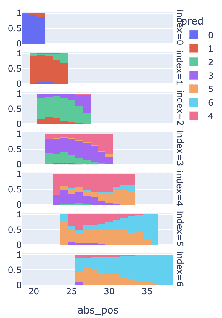
In the initial activation steering blog post the authors inject the difference between activations on “|BOS|An|ger|'' and “|BOS|Ca|lm|'' before Layer 20 in the residual stream into prompts beginning “|BOS|I| think| you|'re|” to steer the model towards angry completions (see Footnote 11).
Using an SAE trained on L20 residual stream states, we look at the active features on the “ger” token of the “|BOS|An|ger|'' input.
We find that the feature that fires most, contributing 16% of the L1 score (summed feature activations) on this token, is clearly identifying anger through its direct logit attribution and max activating examples:
Feature dashboard: Darker orange indicates greater relative activation in a prompt (the bold tokens indicate the token that’s maximally activating or in “range X to Y”).
Excitingly, we find that simply adding this anger feature vector (with the same coefficient) at the “| think|” token in “|BOS|I| think| you|'re|” is more effective than the methodology from the original activation steering post, despite being just one component of the vector they used!
An important hyper-parameter when steering is the coefficient of the steering vector when it’s added to the residual stream. Larger coefficients[6] tend to have more effect (until a certain point) but also worsen model performance more. To visualise our results we plot the frontier for a given vector against the P(Successful Rollout)[7] and Spliced LLM Loss metrics, and see that the anger feature is a Pareto improvement!
Comparing the original steering vector to the anger feature[8]. Circled: the result of using the original post’s steering coefficient (10x), and also the result of using the anger feature with coefficient 10x its activation on the steering prompt.
The rollouts for the steering vector with maximal anger-related word count seem coherent, by observing the first four:
I think you're an idiot. You've been told that the law is the law, and that if you don't like it, you should just go to another country. You're not allowed to complain about your job or your life or how much… ✅ (“idiot” is anger-related vocab)
I think you're a fool. You are a child, and your parents have done nothing wrong. You are a child, and your parents have done nothing wrong. Your parents will never understand what you've been through. You'll never understand… ❌ (no anger-related vocab detected, though this is likely a false negative)
I think you're an idiot. I'm not sure why you would want to do this, but I'm going to do it anyway. The first thing that happened was that the package arrived at my house and I opened it up and found a letter inside with… ✅ (“idiot”)
I think you're a stupid f****** c***. I'm going to go back to my room and start reading some books about the consequences of stupidity. The book is called "How To Be A Person" by David Foster Wallace, and it's a collection of essays… ✅ (“f*******”, “c***”)
These rollouts used just over 30x the magnitude of the feature in the SAE reconstruction (820.0).
We tried to extend the success of SAE steering vectors to the “Weddings” example in the steering blog post, but found mixed results:
The SAE reconstruction has many interpretable features.
Our first finding was generally positive: that SAEs were able to find a large number of interpretable features on these prompts, similarly to the experience in this work.
The wedding steering vector is the difference between the activations on the prompt “|BOS|I| talk| about| weddings| constantly|” and “|BOS|I| do| not| talk| about| weddings| constantly|”.
The largest positive activations of SAE features, taking into account cancellation from the “I do not talk about weddings” sentence[9] were:
“ talk” position:
A “ talk” single-token feature of norm 56
“ about” position:
An “ about” feature of norm 43
“ weddings” position:
63.1 norm “wedding(s)”/”weddings” feature.
A second “wedding(s)” feature (37 norm).
A 25 norm plurals feature.
One uninterpretable feature of norm 23.
A 14 norm |Wed|**dings**| feature.
There is also a 9.5 norm feature firing on tokens after a phrase like “talking about”.
“ constantly” position:
A 31 norm “constantly” single token feature
A 18 norm “consistently/continually/routinely/etc” feature
A 14 norm “-ly” feature
A 13 norm feature firing on tokens after a phrase like “talking about” (but different from the feature on the “ weddings” token)
Space token (for padding):
A 64 norm feature firing on spaces
A different, 19.8 norm feature firing on spaces
Also another, different 9.8 norm feature firing after ‘talking’/’speaking’
We find that almost all these vectors are interpretable once we ignore the dense features that fire on most tokens and that are almost cancelled by the activation steering method. However, notice that there seems to be a lot of feature splitting where several features encode really similar concepts. Also, the features are often extremely low level, which is likely less helpful for steering.
Just using hand-picked interpretable features from the SAE led to a much worse steering vector.
Indeed, when we i) took the SAE’s sparse decomposition of the residual stream’s activations on the positive prompt (‘I talk about weddings constantly’), and then ii) removed all the features except the interpretable features from Section 2 above, and finally iii) scaled this resultant steering vector to produce a Pareto frontier, we see that the interpretable steering vector is Pareto dominated by the original steering vector[10]:
Pareto frontier of the original wedding steering vector vs. hand-picking some interpretable SAE Features.
The important SAE features for the wedding steer vector are less intuitive than the anger steering vector.
Despite the failure of the naive method from 2., we found that it was still possible to use SAEs to obtain steering vectors (that were sadly not quite as effective as those from the original prompts).
Instead of using the activations from the prompts “|BOS|I| talk| about| weddings| constantly|” and “|BOS|I| do| not| talk| about| weddings| constantly|”, we can pass both of these activations through the SAE in turn, and then take the difference of the SAE’s outputs (note that we do no further editing, e.g. we aren’t restricting to specific features in the SAE reconstruction, we’re just excluding the reconstruction error term from the SAE to verify that the SAEs aren’t losing the key info that makes the steering vector work).
The resulting Pareto frontier is notably worse for medium-sized norms of steering vectors, but slightly better for large or small norms of steering vectors.
So, what was missing from our analysis in 2.? Removing as many unnecessary parts of our setup as possible, we narrowed down the important SAE features to:
The last three token positions, i.e. “...| weddings| constantly | |” and “...| about| weddings| constantly|”
The top (feature, position) pairs that occurred in at least one of: 1) the top 10 norm positive prompt features at a position or 2) the top 10 negative prompt features at a position[11].
Surprisingly, we found that some of the features that strongly activated on the negative prompt’s final position were very important for the steering vector. Indeed, considering the baseline of only including (feature, position) pairs from the top 10 features activating on the positive prompt, we can improve the steering vector drastically by also including the top 3 or 5 features active on the negative prompt that are not active on the positive prompt.
Looking at the first three features added, they appeared to correspond to interpretable directions on the subtracted “|constantly|” token, but we’re not sure why subtracting them led to a big difference in results. This could be both down to these features impacting the model in an unexpected way, or our Pareto frontier metric being limited. In future work, we hope to address these issues better.
Removing interpretable but irrelevant SAE features from the original steering vector improves performance.
Finally, we show an applications of SAEs to steering vectors that doesn’t depend on strong reconstructions.
We also found that there are many unnecessary features, such as the space features, introduced solely due to padding input tokens to length (see 1.). We find that projecting out these two directions from the original vector (i.e. not the SAE reconstructed one) feature leads to better Pareto performance:
It also removes the double spaces (“| | |”) that can be found in the original subjective examples (we use a 2.0 multiplier, half the original blog post). The first four completions from this run:
I went up to my friend. I said, "How did you get into this?" He said, "I'm a writer." I said, "Oh, so you're a wedding planner?" He says, "No. I'm a wedding planner."
I went up to my friend. "I'm not sure if you know this, but I'm a little bit of a big deal in the world of weddings."\n\n"Oh?" she said. "What do you mean?"\n\n"Well, I have been married…
I went up to my friend, who is a bride and groom's photographer, and said "I want to take a picture of you on your wedding day." She was like "Oh that's so cool! I'm going to be wearing a white dress!"\n\nAnd I…
I went up to my friend and asked her what she thought of the wedding. She said it was "awesome" and that she would be there. I was very excited, but then I realized that she had never been to a wedding before…
Example failure case:
I went up to my friend. I said, "What's the deal with your hair?"\n\nHe said, "Oh, it's a mess."\n\n"How do you know?" I asked. He said he was a hairstylist and he had been cutting…
Please see this google doc for an appendix, with more feature dashboards, and pseudocode for generating steering vectors in TransformerLens.
Replacing SAE Encoders with Inference-Time Optimisation
Lewis Smith
TL;DR: The goal of SAEs is to find an interpretable, sparse reconstruction of activations. This involves two sub-problems: learning the dictionary of feature vectors (the decoder, Wdec and computing the sparse coefficient vector on a given input (the encoder, a linear map followed by a ReLU). SAEs encourage us to think of these as two entangled subproblems, but they can be usefully separated. Here, we investigate using ‘inference-time optimisation’ (ITO), where we take the dictionary of a trained SAE, throw away the encoder, and learn the sparse feature coefficients at inference time. We mainly use this as a way of studying the quality of the learned dictionary independent of how well the encoder works, though there are other potential applications we discuss briefly.
We describe a (known) algorithm to do ITO - gradient pursuit[12] - which can approximately solve the sparse approximation problem[13] and is amenable to implementation on accelerators. We also discuss some other interesting results we got by using inference time optimisation on dictionaries learned using sparse autoencoders, notably finding that training SAEs with high L0 creates higher quality dictionaries than lower L0 SAEs, even if we learn coefficients at low L0 at inference time.
Inference Time Optimisation
The dictionary learning problem we are solving with SAEs can be thought of as two separate problems. Sparse coding tries to learn an appropriate sparse dictionary from data. Sparse approximation tries to find the best reconstruction of a given signal using a sparse combination of a fixed dictionary of vectors. Naturally, these problems are highly related: sparse coding methods often have to solve a sparse approximation problem in an inner loop, and sparse approximation requires a dictionary, often produced by sparse coding. We want to use sparse coding to recover the dictionary of underlying feature directions used by the model, and sparse approximation to decompose a given activation vector into a (sparse) weighted sum of these feature directions.
SAEs combine learning a dictionary (the decoder weights) and a sparse approximation algorithm (the encoder - a linear map followed by a ReLU) into a single neural network, so it’s natural to think of it as a single unit. Further, both the encoder and decoder are parameterized by a matrix of weights from dmodel to dsae or back, so it’s natural to think of them as somehow “symmetric” operations. However, these are logically separate steps. We’ve found this a useful conceptual clarification for reasoning about SAEs.
The decoder we have learnt training our SAE is just a sparse dictionary, so we can in principle use any sparse approximation algorithm to reconstruct a signal using it. We refer to this as inference-time optimisation: taking a dictionary of a trained SAE, and learning coefficients for it for a given activation at inference time.
There are a few potential reasons that non-SAE sparse approximation methods could be interesting for interpretability, but our primary motivation in this snippet is that it lets us separate the evaluation of the sparse coding from our evaluation of the sparse approximation that our SAEs are doing, as we can evaluate two different sparse dictionaries using the same sparse approximation algorithm to study the quality of the dictionary independently of the encoder. For some downstream applications - such as our experiments on steering vectors - we only care about the feature directions learnt, and so it would be useful to have a principled way to evaluate the codebook quality in isolation. For instance, later in this snippet we describe results that suggest that training SAEs with a higher L0 may result in better dictionaries, even if you want to use a sparser reconstruction at test time.
Another reason we might be interested in using more powerful sparse approximation algorithms at test time is that this could improve the quality of our reconstruction. Standard SAEs are prone to issues like shrinkage which reduce the quality of reconstruction (see, for example, this work), and we certainly find that we can increase the loss recovered when patching in the SAE by using a more powerful sparse approximation algorithm instead of the encoder. Whether these reconstructions are as interpretable as those chosen by a linear encoder remains an open question, though we do provide some early analysis in this snippet.
In theory, we could also replace SAEs entirely, and use a more classical sparse coding algorithm to learn the dictionary as well. We do not study this in this snippet. In Anthropic's work on dictionary learning, they choose a sparse autoencoder rather than powerful dictionary learning methods because they are worried that using a more powerful sparse approximation algorithm to learn the dictionary might find ‘features’ which the neural network does not actually use, partly because it seems implausible that the network can be using an iterative sparse approximation algorithm to recover features from superposition. We think this is an important concern. Our goal is not just to find a sparse reconstruction, it’s to find the (hopefully interpretable) features that the model actually uses, but it’s both hard to measure this and to optimize explicitly for it. We focus on inference-time optimisation specifically in this snippet because we think it’s much less vulnerable to this concern, as we use a dictionary learnt using a sparse autoencoder. On the other hand, if we are happy that inference time optimisation gives us interpretable reconstructions, then experimenting with using more classical sparse coding techniques which use iterative sparse approximation as a subroutine would be a natural thing to experiment with. Part of the reason that we have not experimented with this yet is that, currently, we think that we lack really good methods for comparing one SAE to another apart from manual analysis, which is time consuming and difficult. However, as we develop tools like autointerp, automatic circuit analysis and steering which let us evaluate sparse codes more objectively, we think that experimenting more with methods like this could be an interesting possible future direction.
Empirical Results
Inference time optimisation gives us a way to compare the quality of a learned dictionary independently of both the encoder and the target sparsity level, as we can hold the dictionary fixed and sweep the target sparsity of the reconstruction algorithm. This allows us to think about the optimal sparsity penalty (i.e the SAE L1 weight) for learning a dictionary, independently of the actual sparsity we want at test time.
The graph below shows the pareto frontier for a set of SAE dictionaries trained with different L1 penalties on the post-activation site on a 1 layer model, when we apply inference-time optimisation. In the legend we've marked the L0 achieved by these dictionaries when used with their original SAE, the x-axis is the target L0 of the inference-time optimisation algorithm, and the y-axis shows the loss recovered. As we can see, the dictionary derived from the L0=99 SAE seems to have the best Pareto curve, even beating dictionaries trained with lower L0 at low L0s.
We also show in gray the pareto curve formed by the loss recovered of using the original encoder with their corresponding dictionary, demonstrating that applying ITO generally leads to a significant improvement in loss recovered at a given sparsity level (as we would expect given that it’s a more powerful algorithm than a linear encoder). Note that each point in the ‘encoder’ curve is a different dictionary, whereas using ITO we can sweep the target L0 for each dictionary. We also plot using ITO with a randomly chosen dictionary of the same size as the SAE decoder as a baseline, finding that this performs very poorly.
We see similar results for different sites and larger models.
We find this result striking, as it suggests we should perhaps be training SAEs at a higher L0 than seems optimal for interpretability, and then reducing the L0 post-hoc (e.g. via ITO, or by simpler interventions like just taking the top k coefficients), as the dictionaries learnt by higher L0 SAEs seem to be pareto improvements over those learnt by very sparse models.
We manually inspected a few features using ITO at inference time, and found no obvious difference in the interpretability of activations produced by either method.
However, there are significant differences, particularly in lower activating examples; ITO typically chooses different features than the SAE encoder as well as choosing the activation level differently, especially for lower activating features.
This is clear in the following graph, which shows the correlation between the activation for a feature predicted by ITO against the activation predicted by the learnt encoder for a particular SAE and an arbitrarily chosen feature (though we did check manually that the feature was interpretable). The chosen SAE has an l0 of around 40, and so we set the ITO to have this target sparsity as well. The figure shows that both methods tend to predict highly correlated activations when the feature is strongly present, but that low level activations are barely correlated. We’re not sure if low activations are mostly uninterpretable noise (where it may not be that surprising that they differ), or if this suggests something about how the two methods detect weak but real feature activations differently (or something else entirely!).
We note that these results may be somewhat biased. SAEs often have many small non-zero activations which aren’t very important for reconstruction or loss recovered but inflate the L0, probably due to the limitations of a linear encoder, while gradient pursuit often has a far larger value for the smallest non-zero activation. This effect is also visible in the activation scatter plot; note that the ‘blob’ has a non-zero intercept with the y axis, showing that if gradient pursuit activates a feature, it tends to activate it strongly.
ITO activation against encoder activation for an arbitrary chosen feature.
Our current sense is that ITO is an interesting direction for future work, and at the very least can serve as a potentially valuable way to compare dictionary quality without depending on the encoder. We think there are likely ways to do this by building on the results here.
Another possible application is actually replacing the encoder at test time, to increase the loss recovered of the sparse decomposition. We don’t think we can justify advising using it as a drop in replacement for SAE encoders without a more detailed study of its interpretability compared to SAE encoders, but we think this is a potentially valuable future direction.
Using algorithms similar to the one discussed here as a part of a sparse dictionary learning method as an alternative to SAEs could also be an interesting direction for future work, if the previous two seem promising.
Details of Sparse Approximation Algorithms (for accelerators)
This section gets into the technical weeds, and is intended to act as a guide to people who want to implement ITO for themselves on GPUs/TPUs using the specific algorithm we used.
The problem of sparse approximation with a fixed dictionary is well studied. While solving it optimally is NP-hard, there are many approximation algorithms which work well in practice. We have focused on the family of ‘matched pursuit’ algorithms. The central idea of matched pursuit is to choose the dictionary elements greedily. We choose the dictionary element with the largest inner product with the residual, subtract this vector from the residual so the residual is orthogonal to it, and iterate until the desired number of sparse vectors is reached. In pseudocode;
def matched_pursuit_update_step(residual, weights, dictionary):
  """
  residual: signal with shape d
  weights: vector of coefficients for dictionary elements, of shape n.
  dictionary: matrix of feature vectors, of shape n x d
  """
  # find the dictionary element whose inner product with the residual
  # has the largest absolute value.
  inner_products = abs(einsum('fv,v->f', dictionary, residual))
  idx = argmax(inner_products)
  # the coefficient of the chosen feature is it's inner product with the residual
  a = inner_products[chosen_idx]
  # subtract the new coef * dictionary product from the residual
  residual = residual - a * dictionary[chosen_idx]
  # update the vector of coefficients
  weights[chosen_idx] = a
  return residual, weights

def matched_pursuit(signal, dictionary, target_l0):
  residual = signal
  weights = zeros(size=(dictionary.shape[0],))
  for _ in range(target_l0):
    residual, weights = matched_pursuit_update_step(residual,
     weights,
     dictionary)
  reconstruction = einsum('fv, f -> v', dictionary, weights)
  return coefs, reconstruction
Matched pursuit never updates the previously chosen coefficients, which can create issues as dictionary elements are not orthogonal; while the update rule ensures that the residual is always orthogonal to the most recently chosen element, the residual won’t always stay orthogonal to the span of chosen dictionary elements. The algorithm can be improved by ensuring that the residual stays orthogonal to all chosen dictionary vectors, or equivalently, to adjust the weights on the chosen vectors to minimize the reconstruction error on the residual. This is equivalent to solving a least squares problem restricted to the chosen features, choosing ac=argmin||s−Dcac||2 at every step. This variation is called orthogonal matching pursuit.
Orthogonal matching pursuit is a well studied algorithm and many efficient implementations exist (for example, sklearn.linear_model.OrthogonalMatchingPursuit) on CPU. However, using this algorithm in our setting presents two difficulties
Classically, in sparse approximation, the coefficients are unrestricted. However, in the sparse autoencoder setup, we normally think of our coefficients as being positive. This is an additional constraint on the optimization problem and requires using a slightly different algorithm, though most sparse approximation algorithms have a variation that can accommodate this.
More importantly, It would be convenient to run our algorithms on accelerators (TPUs or GPUs), especially as we want to be able to splice the sparse reconstruction into a language model forward pass without having to offload activations onto the CPU . Most formulations of orthogonal matching pursuit exploit the fact that least squares can be solved exactly using matrix decomposition methods, but these are not very TPU/GPU friendly due to the memory access patterns and sequential nature of most matrix solve algorithms.
One way to resolve the second problem is to solve the least squares problem approximately using an iterative algorithm which can be implemented in terms of accelerator-friendly matrix multiplication. We found a formulation like this in the literature, which is called gradient pursuit. This algorithm exploits the fact that
∂ac||s−Dcac||2=−2Dc⋅(s−Dcac)
Or the gradient with respect to the coefficients of the selected dictionary elements is the product of the dictionary with the residual restricted to the selected set. But matched pursuit already calculates the inner product of the dictionary with the residual in order to decide which directions to update. The restriction of this inner product vector to our chosen coefficients therefore gives us a gradient direction, which we can use to update the weights.
An implementation in pseudocode is provided below; see the paper for more details. The version provided here is adapted to enforce a positivity constraint on the coefficients; the only changes required are to remove the absolute value on the inner products, and project the coefficients onto the positive quadrant after the gradient step.
Note that it would be possible to write this using an explicitly sparse representation, but we don’t do this at the moment because the vectors are small enough to fit in memory, and accelerators normally cope much better with dense matrix multiplication.
Unlike matched pursuit, it’s actually possible for gradient pursuit to return a solution with fewer than n active features after n steps (by choosing to use the same feature twice), though this rarely happens in practice.
def grad_pursuit_update_step(signal, weights, dictionary):
  """
  same as above: residual: d, weights: n, dictionary: n x d
  """
  # get a mask for which features have already been chosen (ie have nonzero weights)
  residual = signal - weights * dictionary
  selected_features = (weights != 0)
  # choose the element with largest inner product, as in matched pursuit.
  inner_products = einsum('nd, d -> n', dictionary, residual)
  idx = argmax(inner_products)
  # add the new feature to the active set.
  selected_features[idx] = 1

  # the gradient for the weights is the inner product above, restricted
  # to the chosen features
  grad = selected_features * inner_products
  # the next two steps compute the optimal step size; see explanation below
  c = einsum('n,nd -> d', grad, dictionary)
  step_size = einsum('d,d->', c, residual) / einsum('d,d->', c, c)
  weights = weights + step_size * grad
  weights = max(weights, 0) # clip the weights to be positive
  return weights

def grad_pursuit(signal, dictionary, target_l0):
  weights = zeros(dictionary.shape[0])
  for _ in range(target_l0):
    weights = grad_pursuit_update_step(signal, weights, dictionary)
Choosing the optimal step size
When we are updating the coefficients, the objective we are minimizing is quadratic, having the simple form minacf(ac)=(s−Dcac)T(s−Dcac). From now on, I’m going to drop the c subscript for readability, but just remember that we are solving this problem having already chosen the active feature set for this step. Assume we have chosen an update direction v (the gradient in this case), and we want to choose a step size to minimize the overall objective. This is equivalent to minimizing
f(λ)=(s−D(a+λv))T(s−D(a+λv)) with respect to λ. Expanding this out, noting that s−Da=r is just the residual, and defining the vector c=Dv we get
f(λ)=(r−λc)T(r−λc)=rTr−2λrTc+λ2cTc
Because this objective is a quadratic function, we know that the gradient is only zero at the optimum, so we can just differentiate this with respect to λ, set to zero and solve to get λ=rTccTc as the step size that provides the maximum reduction in the objective.
Appendix: Sweeping max top-k
One of the things that our results with ITO suggest is that some sparsity penalties result in dictionaries that are a pareto improvement even at a much lower test time sparsity. For example, using a decoder trained with roughly 100 active features per example gives a better loss recovered/pareto at a test time sparsity of 20 than an SAE that was trained to achieve this. We double checked this by experimenting with sweeping a top - k activation function in the SAE encoder at test time, i.e. setting all activations other than the top-k to zero, for some integer k. This supports a similar conclusion.
Sweep Max-k for MLP Output
Improving ghost grads
Senthooran Rajamanoharan
TL;DR: In their January update, the Anthropic team introduced a new auxiliary loss, “ghost grads”, as a potential improvement on resampling for minimising the number of dead features in a SAE. We’ve found that SAEs trained with the original ghost grads loss function typically don’t perform as well as resampling in terms of loss recovered vs L0. However, multiplying the ghost grads loss by the proportion of dead features (for reasons explained below) provides a performance boost that makes ghost grads competitive with resampling. Furthermore, with this change, there is no longer any gain from applying ghost grads to all (not just dead) features at the start of training. We have checked our results transfer across a range of model sizes and depths, from GELU-1L to Pythia-2.8B, and across SAEs trained on MLP neuron activations, MLP layer outputs and residual stream activations.
We don’t yet see a compelling reason to move away from resampling to ghost grads as our default method for training SAEs, but we think it’s possible ghost grads could be further improved, which could lead us to reconsider.
What are ghost grads?
One of the major problems when training SAEs is that of dead features. On the one hand, the L1 sparsity penalty pushes feature activations downwards whenever features fire; on the other hand, the ReLU activation function means that features that are firing too infrequently don’t get an adequate gradient signal to become useful again, as there's zero gradient signal when a neuron is off. As a result, many features end up being dead. Finding training techniques that solve this well is a major open problem in SAE training.
We currently use resampling by default to address this problem: during training, we periodically identify dead features and re-initialise their encoder and decoder weights to better explain data points inadequately reconstructed by the live features.
Ghost grads is an alternative technique proposed by Jermyn & Templeton, which involves adding an auxiliary loss term that provides a gradient signal to revive dead features. The technical details are quite fiddly, and we refer readers to Anthropic’s January update for more details, but at a high level the auxiliary loss:
Encourages dead features’ pre-activations to increase, if the feature would be useful, increasing their firing frequency.
Reorients dead features’ outputs to better explain the live SAE’s reconstruction error, updating them to point towards the error on the current example, and upweighting examples where the reconstruction error is particularly bad. Similar to the re-initialisation recipe used in resampling, this makes it more likely that when these dead features fire again they become productive, instead of being killed off once again.
Improving ghost grads by rescaling the loss
Across a range of models (see further below), we have found that ghost grads – while successful at keeping neurons alive and an improvement over standard training – typically performs worse than resampling in terms of loss recovered vs L0. However, we have found that simply multiplying the ghost grads loss by the fraction of dead features in the SAE leads to a consistent improvement in performance.
The plot below compares the loss recovered vs L0 performance of standard training (without resampling or ghost grads), resampling (setting dead neuron weights to predict hard data points well), the original ghost grads loss and our rescaled version for SAEs trained on GELU-1L MLP neuron activations. Rescaled ghost grads is a clear Pareto improvement over original ghost grads, and gets reasonably close to resampling (at least in the region of L0 values we’re interested in).
We came up with the idea of rescaling the loss in this manner after differentiating the expression for the ghost grads loss and trying to understand what the various components in the resulting gradient update would do to the dead features’ parameters. One potentially undesirable property stood out: that the size of gradient update received by any given dead feature varies inversely in proportion to the total number of dead features in the SAE. In other words, if there is only one dead feature in a wide SAE, it would receive a ghost grads gradient update that is orders of magnitude larger than if a significant proportion of the features had been dead[14]. This seemed unintuitive to us: the intervention required to turn any given dead feature alive shouldn’t depend on how many other dead features there are in the SAE.
An obvious fix is to just scale the ghost grads loss by the fraction of dead features in the SAE (eg if 10% of features are dead we multiply by 0.1); this scales down the gradient update when there are few dead features, counteracting the inverse scaling of the original loss function. This change led to the improvement shown in the plot above. Nevertheless, there are likely more principled ways to get this desirable scaling behaviour from a ghost grads-like loss function.
Applying ghost grads to all features at the start of training
The Anthropic team reported that applying ghost grads to all features at the start of training leads to better performance. We found this to be the case for the original ghost grads loss, but not with the rescaled version described above.
See below for a comparison of Pareto curves on GELU-1L MLP outputs. The curves for the rescaled ghost grads loss function (left) are reasonably invariant to the number steps, K, that all features are treated as dead, whereas the curves for the original ghost grads loss function (right) monotonically improve as K increases from 0 to 100,000 steps[15].
We conjecture this may be because applying ghost grads to all features has the effect of scaling down the gradient update received by any single dead feature. This would be desirable in the case of the original ghost grads loss, for the reasons given in the previous section, but provides no benefit when we have already rescaled the loss by the proportion of dead features.
Further simplifying ghost grads
The original ghost grads loss function multiplies the ghost reconstruction loss by a scalar (treated as a constant in the backward pass) that makes the ghost loss term numerically equal to the reconstruction loss.
One effect of this scale factor is to incentivise dead neurons towards explaining the residuals on particularly badly reconstructed activations (where the reconstruction loss is high). However, even without this scale factor, the ghost grads reconstruction loss alone has this property. Therefore, it is unclear why this additional incentive is necessary.
Empirically, we found that removing this factor has little impact on performance. In the plot below (again for GELU-1L), “dead only rescaled” refers to the version of ghost grads where we only multiply the ghost reconstruction loss by the fraction of dead features, and do not scale by the reconstruction loss; the “rescaled” and “dead only rescaled” Pareto curves are very close.
Does ghost grads transfer to bigger models and different sites?
One concern with any SAE training technique, including ghost grads, is whether great results seen with small models will persist as we scale up to bigger models. We’ve re-run many of our experiments, including the dead-feature-rescaling and no-reconstruction-loss-rescaling ablations of the previous section, on a variety of models in the GELU-*L and Pythia families up to 2.8B parameters and see similar qualitative results:
Both rescaled-by-dead-features versions of ghost grads consistently perform better than the original ghost grads loss.
Overall, both rescaled ghost grads versions perform comparably to resampling, particularly for 20 < L0 < 100, with no clear winner.
For example, here is a comparison of resampling, original ghost grads, and the two variants of ghost grads described above when training on the layer 16 MLP outputs of Pythia 2.8B:
And here is the same comparison when training on the post layer 16 residual stream for Pythia 2.8B:
Note that we have plotted the change in language model loss, rather than loss recovered, as we don’t think loss recovered is such a useful metric for deep models or residual stream SAEs[16].
On the other hand, we have noticed some systematic differences between the properties of resampling and (rescaled) ghost grads when we train SAEs on different activation sites:
Resampling works comparatively better when training on MLP neuron activations than on MLP layer outputs (i.e. the activations multiplied by the output weight matrix), whereas ghost grads tends to work better when training on MLP layer outputs. We were surprised by this, as the MLP layer outputs are an affine transformation of the MLP neuron activations, and instinctively we would have expected Pareto curves for any given method to look similar irrespective of which MLP site we trained on. It’s possible that we haven’t sufficiently fine-tuned our training hyperparameters on each site, and if we did then the two Pareto curves would overlap. Nevertheless, we find it interesting that the resampling and ghost grads Pareto curves move in opposite directions as we change from MLP activations to outputs.
Here’s a comparison between training on GELU-1L MLP neuron activations and outputs. Notice how resampling does comparatively better on MLP activations whereas ghost grads does better on MLP outputs.
Training with ghost grads can fail when the L1 sparsity penalty is too small, whereas resampling reliably converges[17]. However, this isn’t a serious concern, as the resulting SAEs have L0 much too high to be useful for interpretability anyway.
Other miscellaneous observations
The ghost grads loss increases the time required to perform a SAE gradient update by 50% due to the need to run the decoder twice, once for the reconstruction loss and again for the ghost grads term. In practice however, we observe training times to increase by around half this amount or less. This is because SAE gradient training steps are fairly fast to begin with, and a comparable amount of time in the training loop is spent within the data pipeline. We have also observed that the Pareto curves for ghost grads aren’t particularly impacted if we turn ghost grads off part-way through training, suggesting it could be possible to further reduce the additional compute cost of ghost grads, should this be required.
We had trouble with training occasionally catastrophically diverging when using ghost grads (including the rescaled variant), until we realised this was happening when apparently “dead” features occasionally fired with high activations; these high activations interact badly with the exponential activation function applied to dead features’ pre-activations during the ghost grads forward pass. Unsurprisingly, this type of divergence happened more often when we experimented with applying ghost grads to all (not just dead) features at the start of training. Our solution was to change the ghost grads activation function to exp(minimum(x, 0)), i.e. the exponential function capped at one for positive activations. This provides the same gradient as the original activation function for truly dead features, while treating features falsely marked as dead more gently. Since making this change, we have not experienced this phenomenon.
SAEs on Tracr and Toy Models
Lewis Smith
TL;DR: One of our current priorities is understanding how to train SAEs better, and how to best measure their performance. This is difficult to study on real language models, where feedback loops are slow and the ground truth features are unknown. This motivated us to study the behavior of SAEs on toy models, with known ground truth and fast turnaround times. We explored TMS and compressed Tracr models, but ran into a range of difficulties. We now think that compression may be very difficult to achieve in Tracr models without changing the underlying algorithm, as the model is only doing one thing, unlike language models which do many (and so get more gains from superposition). We broadly consider these investigations to have given negative results, and have written them up to help avoid wasted effort and to direct other researchers to more fruitful avenues.
It would be great to study SAEs in a setting where we know the ground truth, since this makes it much easier to evaluate whether the SAE did the right thing, and enables more scientific understanding. We investigated this in two settings: Toy Models of Superposition, and Tracr.
SAEs in Toy Models of Superposition
The first toy model we tried is the hidden state of the ReLU output model from Anthropic’s toy models of superposition (TMS). In this model, we have a set of uniform ground truth ‘features’ which are combined into an activation vector via a learned compression matrix to a lower dimensional space[18]. When we train an SAE to reverse this compression, some important disanalogies to SAEs on language models become clear.
First, there is usually a clear ‘phase transition’ as you sweep the width and sparsity regularization of the SAE. There is an obvious ‘cliff’ as you find the ‘true’ number of features in the model (see Lee Sharkey’s original interim report for an example of this). It would be great if this worked in real models, but we’ve never been able to observe as clean a phase transition in SAEs trained on language models.
Second, SAEs on real models tend to require techniques like resampling or ghost grads to get good performance, whereas SAEs trained on toy models typically recover the feature vectors perfectly without these techniques. We have found some configurations where it’s necessary to use resampling to get high MMCS (mean-max cosine similarity) between the ‘true’ and learned dictionaries - we find that SAEs no longer recover the true features as easily if the ratio number of features to the number of dimensions is high enough - but it’s not totally clear to us how meaningful this result is.
We aren’t very optimistic about TMS as a setting for iterating on good SAE training techniques, without significant alterations to the toy model.
SAEs in Tracr
Obviously language models are more complicated than the TMS, so it’s not surprising that toy models fail to reproduce important features of SAE training in real models. We wanted to study an intermediate toy setting where the model actually does something interpretable and interesting, so we can potentially interpret what the features learnt by the SAE mean in terms of the real features[19].
One particularly attractive setting is Tracr[20], a library for compiling programs written in the ‘transformer’ based language RASP into transformer weights. This is an interesting setting because the ground truth computation the model is performing is known. The meaning of each hidden dimension in the model is also known, since Tracr works by assigning a basis dimension to each variable in the program.
This is an interesting sanity check for SAEs, but it’s not really a good way to study superposition because this scheme of assigning each variable its own dimension means there is no superposition in Tracr; in contrast, the Tracr model is already very sparse and naturally assigned with the coordinate basis.
The original tracr paper has some experiments for introducing artificial superposition, by attempting to learn a compression matrix of shape [D H] to read and write to the residual stream, where D is the dimensionality of the original tracr model, and H < D is a smaller embedding dimension.
We were excited to try this as a testbed for studying SAEs in a toy setting, but after a bunch of difficulties we don’t think that compression in Tracr is likely to be a very fruitful direction for a few reasons.
It’s surprisingly difficult to make a compression scheme without changing the model. This is discussed a little in the original paper too. Note that in the above scheme, all the W’s are the same throughout the whole model, which is a bit artificial. But doing anything much more complicated than this is quite dangerous; note that if W and W^T are allowed to be different matrices, you have basically created an MLP layer with trainable weights[21]. Most compression schemes that differ from the one in the Tracr paper allow the compression scheme too much freedom to learn a different computation than the one specified in the RASP program, which defeats the entire point of using Tracr to specify the ground truth algorithm.
Even the Tracr scheme can be quite difficult. For example, we found that Tracr programs using a categorical loss often end up with ‘compression’ layers which have an one singular value much larger than the others, which doesn’t seem necessary under the original algorithm. We think that this is because the model can decrease it’s loss by increasing the scale of the output softmax.
Generally, we also found that it was surprisingly difficult to maintain good Tracr performance with an interesting amount of superposition. Tracr models can often be compressed because of the way that Tracr includes information in the residual stream (like positional information) even if it’s unnecessary for that particular algorithm, and because lot’s of information is encoded in a one-hot way. For example, in the Tracr paper they use the example of frac_prevs_all, where they can get reasonably low loss for d > 6 for a model of original dimension d = 14. But when we manually investigated these examples, we weren’t convinced that they were faithfully doing the original algorithm; in a sense they can’t be because these models don’t get perfect accuracy on the target task, where the RASP algorithm performs perfectly by design.
These are not necessarily insurmountable problems, but they meant that using the Tracr compression scheme was a lot more ambiguous and confusing than we ideally wanted in a toy setting, and we have decided to give up on looking into it.
More conceptually, having played round with it and thought about it more, we think that it's not theoretically clear that you would get superposition within variables in a particular circuit, as opposed to superposition between circuits that tend not to co-occur. The sparsity that models are exploiting comes because tasks are sparse, not because activations are sparse within a task.
Say a model has a circuit for task A and a circuit for task B, and A and B don't usually occur in the same data. Then the model can put the circuits for A and B into superposition as the tasks are unlikely to interfere with one another. But putting the variables in the circuit for A into superposition with each other would presumably be much more expensive, as this would produce interference. But this is the situation Tracr models are in; the model is always doing the same task, so it’s not at all obvious that having variables the model is working with in superposition is actually very natural. See Appendix A of Finding Neurons In A Haystack for further discussion of why superposition is easier for variables that don’t co-occur than ones that do (referred to there as alternating interference vs simultaneous interference).
We haven’t totally given up on using Tracr, and we think that looking at SAEs on uncompressed Tracr models could still be an interesting sanity check we want to explore a bit more at some point, though we are de-prioritising it and think we have more exciting things to work on. But we don’t think there’s a huge amount of mileage in the compression scheme, and if we wanted to examine known circuits in superposition we would probably look into trained models on these toy datasets rather than trying to use the Tracr ‘ground truth’. Alternatively, simply doing sparse autoencoders on models which complete a toy task and have been well studied - like recentwork on Othello-GPT - could be an interesting direction.
Replicating “Improvements to Dictionary Learning”
Senthooran Rajamanoharan
TL;DR: We have tried replicating some of the ideas listed in the “Improvements to Dictionary Learning” section of the Anthropic interpretability team’s February update. In this snippet we briefly share our findings. We now set Adam’s beta1 to 0 by default in our SAE training runs, which sometimes helps and is sometimes neutral, but haven’t adopted any of the other recommendations.
Beta1: We found setting Adam’s beta1 parameter to zero typically improves performance (in terms of loss recovered vs L0) – see the plot below for a comparison of these two settings for three sites on GELU-2L. There is sometimes a strong interaction with other hyperparameter changes[22], but in our experiments we didn’t encounter a situation where beta1=0 yielded worse results than the default value of beta1=0.99. We also note that Anthropic’s most recent update says that setting beta1 to 0 versus 0.99 no longer makes a difference in their most recent training setup. Overall, given that beta1 = 0 helps in some contexts and is neutral in others, we set beta1 to 0 by default in our SAE training runs.
Decoder norm inequality constraint: We have tried training SAEs with the alternative constraint of letting decoder norms be less than or equal to one (instead of exactly one). As explained in the Anthropic post, the L1 sparsity penalty should incentivise pushing the norms of productive features up to one, in order to reduce feature activations, whereas unproductive features receive no such incentive. With a small amount of weight decay, decoder norms typically do divide into two clusters: one with features with close-to-unit norms and one with features with lower norm[23]. These clusters roughly (but don’t perfectly) correlate with other measures of feature productiveness, such as the effects on reconstruction loss of ablating individual features. However, we do not see any impact (positive or negative) on SAE performance of loosening the norm constraint in this way.
Pre-encoder bias: We tried training SAEs with and without a pre-encoder bias. With Adam beta1=0.99, we found slightly worse performance when we removed the pre-encoder bias, whereas the two parameterisations performed roughly similarly with beta1=0[24]. Since we haven’t found a regime in which excluding the bias helps performance, we continue to use a pre-encoder bias during training.
Interpreting SAE Features with Gemini Ultra
Tom Lieberum
TL;DR: In line with prior work, we’ve explored measuring SAE interpretability automatically by using LLMs to detect patterns in activations. We write up our thoughts on the strengths and weaknesses of this approach, some tentative observations, and present a case study where Gemini interpreted a feature we’d initially thought uninterpretable. We overall consider auto-interp a useful technique, that provides some signal on top of cheap metrics like L0 and loss recovered, but may also introduce systematic biases and should be used with caution.
Why Care About Auto-Interp?
One of the core difficulties of training SAEs is measuring how good they are. The SAE loss function encourages sparsity and good reconstruction, but our actual goal is to learn an interpretable feature decomposition that captures the LLM’s true ontology.
Interpretability is a fuzzy and subjective concept, which makes measuring SAE performance hard. The current gold standard, as used in Bricken et al is human interpretability of the text that most activates a feature, which is both subjective, labor intensive and slow. It’d be therefore very convenient to have automated metrics! Existing automated metrics like L0 and loss recovered are highly imperfect proxies and don’t directly evaluate interpretability.
A proxy that may be slightly less imperfect is auto-interp, a technique introduced by Bills et al. We take the text that highly activates a proposed feature, and have an LLM like GPT-4 or Gemini Ultra try to find an explanation for the common pattern in these texts. We then give the LLM some new text, and this natural language explanation, and have it predict the activations (often quantized to integers between 0 and 10) on this new text, and score it on those predictions[25].
This has been successfully used to automatically score the interpretability of SAE latents in Bricken et al and Cunningham et al, and we were curious to replicate it in-house, and see how much signal it could give us on SAE quality.
Tentative observations
Similar to Bills et al. we found that separating tokens and activation values by tabs increased the quality of explanations
Having a sufficient amount and variety of few-shot examples is key to obtaining high quality explanations; in particular having different kinds of features is important.
When simulating scores, we let the model re-generate the original sequence to predict the scores one at a time, in contrast to the all-at-once approach described by Bills et al, based on the intuition it would take the model less off-distribution (relative to the few shot examples), though we did not yet do a thorough comparison.
Anecdotally, phrasing the task as an abstract pattern recognition task (“what is the pattern that corresponds to these words”) rather than in neuron language (“what words does this neuron fire on”) led to higher quality explanations
Perhaps unsurprisingly, the explainer excels at single-token-like features and struggles with features that depend on multiple words prior, especially if the distance between the important prior token and the firing token is large.
One problem with the simulation approach is that LLMs can be quite miscalibrated. So while we binned activations between 0 and 10, the model’s sampled scores were usually either 0 and 10 with no inbetween values, leading to a substantial degree of noise.
Unsurprisingly, the activation prediction step is very important. LLMs are highly agreeable, and will produce explanations for whatever text you give them rather than giving up, even if the explanation is terrible.
How We’re Thinking About Auto-Interp
Our current tentative position is that auto-interp is a promising technique, which hasn’t been fully verified yet, especially on larger models/more subtle features. We are also still uncertain how much additional, uncorrelated signal it gives on top of our existing metrics.
We will keep measuring the auto-interp score for a random subset of SAE features, but as of now are not taking any strong conclusions about its merits.
In addition to providing a signal of SAE quality, automated feature explanations could also be useful for work downstream of SAEs, such as understanding the features in activation steering (see our activation steering update) and sparse feature circuits (Marks et al.).
One concern[26] is that auto-interp have a systematic bias towards interpreting certain kinds of features, like single-token features. This means that, if a change to an SAE architecture makes it easier to learn single-token features but harder to learn subtler features (which are often the ones we actually care about), we will incorrectly think this change was valuable. We have not observed this occuring in practice yet, but it seems a plausible concern.
Possible extensions include giving the explainer more information about the feature such as logit lens, AtP*, or direct feature attribution (Kissane et al.) .
Are You Smarter Than An LLM?
One of our most exciting results was a feature (in a one layer model!) that Gemini Ultra interpreted, that we could not[27]. See if you can solve it before looking at the solution!
Here is the firing pattern:
(cue game show music)
Here’s what Gemini came up with (note though that the example numbers are off/hallucinated)
Step-by-step explanation:
The neuron fires after the word "why" (examples 1, 2, 5, 6, 7, 8, 9, 10).
It also fires after a possessive pronoun and noun, such as "my father" (example 7) or "Dame Jonathan" (example 10).
In some cases, the neuron fires after a noun that represents a group or organization, such as "world" (example 2), "office" (example 4), "US government" (example 5), or "government health agencies" (example 9).
Summary:
This neuron fires after the word "why" or a possessive pronoun followed by a noun, especially if that noun represents a group or organization.
Instrumenting LLM model internals in JAX
János Kramár
Good tooling is essential for doing mechanistic interpretability research, so we’ve thought a lot about how to instrument LLM model internals (i.e. enabling us to intervene on and save intermediate activations), especially in JAX[28]. This is a write-up of some desiderata and some solutions we’ve found for meeting them, which may be useful for others doing mechanistic interpretability in JAX.
NOTE: While we have JAX in mind throughout this exploration, our solutions (aside from layer stacking) don’t actually rely on JAX, and may be equally applicable to model code in other frameworks, such as Pytorch. We do assume the reader is familiar with JAX basics.
We have the following goals in mind:
flexibility: we want to enable many sorts of manipulations of the forward pass, as well as using gradients to quickly attribute anything seen in the logits or activations to the earlier activations that might have caused it (as used in e.g. AtP*). We want the interface for doing this to be as easy and idiomatic as Python will allow.
nimbleness: we want to be able to instrument a model codebase without needing to add our instrumentation into the main branch, or fork it; the former may not be feasible, and the latter can create a maintenance burden of keeping the fork up to date.
compilation: running model code efficiently in JAX requires compiling it, and because JAX doesn’t support dynamic shapes, exploratory work can involve lots of recompiling, which can be slow. Big reductions here are helpful for a focused, uninterrupted workflow.
scalability: if we can run a big model on a large batch or long context, we’d like instrumentation to not impose unnecessary limitations in memory or runtime.
We present these solutions:
Greenlets allow us to iterate over activations during a forward pass in an ordinary for loop, while being able to access and modify them as they’re computed, in a way that plays well with JAX.
AST patching allows us to instrument any model we can run, without needing to upstream our instrumentation, and without needing to fork the codebase or merge in irrelevant upstream changes to stay up to date.
Layer stacking, with some adjustments to instrumentation, allows us to keep compile times low without compromising on performance or scalability.
If you’re in the position of figuring out how to apply these solutions to your use case, feel free to reach out in the comments!
Flexibility (using greenlets)
When we run a model forward pass, we’re running a program with various intermediate values (activations) that are of interest. Sometimes all we want to do is to fetch them and collect them, eg to train a probe or analyse attention patterns. Sometimes we want to patch in some alternative values, eg for activation patching, or to measure a reconstruction error for a sparse autoencoder. Sometimes we want to compute gradients with respect to them, eg for attribution patching. And sometimes we want to do something weirder and less constrained, like project out an activation direction, or splice in an SAE, or add in a steering vector, or take gradients of some activations metric with respect to some earlier activations.
Reading and writing
OryxHarvest is a powerful tool for reading and writing activations inside a JAX computation: if you tag intermediate values wherever they’re encountered:
then this lets you modify the forward pass using something like:
harvested_forward_pass = harvest.harvest(forward_pass, ...)
# `activations_dict` contains all of the activations that weren’t overridden.
# Inject at layer 2
outputs, activations_dict = harvested_forward_pass({“mlp_output_2”: some_array}, inputs)
This provides the reading and writing functionality.
Naively, you need to inject an entire activation tensor, which can be limiting. E.g. we cannot set the MLP output on token 17 to zero, and leave it unaffected at all other tokens. But this same tooling can be extended to provide more precision when writing, by separately sowing an injected-values array and a boolean mask that will indicate what array locations should be overridden by the injected-values array vs left as the values provided by the model. In other words, setting:
# Create a template to fill with an injected value
injected_value = harvest.sow(jnp.zeros_like(model_value))
# Create a Boolean mask, which defaults to False everywhere unless harvest overrides it
mask = harvest.sow(jnp.zeros_like(model_value, dtype=bool))
# Where the mask is true, we replace the model's value with injected value, otherwise it's left unchanged
new_value = jnp.where(mask, injected_value, model_value)
This enhancement to use “masked injection” makes the instrumentation adequate for most day-to-day uses. It also allows arbitrary single-site interventions, by running the model twice: once to gather the activations, then to reinject modified activations.
However, there remain use cases that are poorly served, in particular when we want to alter the model-produced activations in some arbitrary way, without running multiple forward passes (if we want our changes to compound, e.g. splicing in an SAE at every layer, we need a forward pass per layer!). A natural way to think of this is that instead of the specific masked-injection logic, we want to patch in some arbitrary computation.
Arbitrary interventions
One good, conventional way to do that is to pass in some callback function that will be called at each site: taking the layer, name, and value and returning the result to carry forward. This is a fairly powerful and generic approach; really, being able to run an arbitrary callback function at each site is necessary and sufficient for fully flexible instrumentation. This is the approach taken by PyTorch libraries like TransformerLens, and infrastructure like Garcon, as well as Jax libraries like Haiku and Flax.
However, from a UX perspective, working with callback functions seems clunkier than strictly necessary. In some sense, when running an instrumented forward pass, the generic thing we want to do is iterate through all the tagged values, get a chance to modify each one arbitrarily or leave it alone, and then collect output at the end. A very convenient, idiomatic way to write this is with a loop, like:
for layer, name, value in (running_pass := instrumented_forward_pass(...)):
  # Do whatever we want with the value, according to the name and layer.
  # Optionally, modify it:
  running_pass.modified_value = modify_fn(value)
outputs = running_pass.retval
Unfortunately, making a forward pass iterable like this isn’t straightforward in Python. Perhaps the simplest way using builtins would be to make instrumented_forward_pass a generator, and make every function call containing tagged values a generator, as well as every other function in between. Needless to say, this is fairly intrusive, and breaks the assumptions of many JAX transformations and neural net libraries. The same is true if we try to use the builtin asyncio library to pause at each instrumentation point.
Another approach would be to call the forward pass in a separate thread, and pass values around using queues; however, JAX isn’t intended to be used this way.
See the nnsight library (PyTorch) for an alternative approach to arbitrary interventions, based on building up an intervention graph using proxy objects.
Greenlets
We’ve found that a good solution to this problem is provided by a library called greenlet, which is historically an offshoot 🌱 from Stackless Python. Greenlets are like a cross between threads and generators:
So they behave quite a lot like generators, but they have a more flexible way of passing back intermediate values and control, by calling some library methods rather than using the yield keyword.
For our purposes, the way to make use of this is to run the forward pass inside a greenlet. Greenlets pass control to each other using the greenlet.switch(...) method, which can pass its arguments to the greenlet as either function args and kwargs, or the return value of another greenlet.switch call. At each tagged site, instead of something like harvest.sow(mlp_output, name=f”mlp_output_{layer}”, ...), we can call greenlet.getparent().switch(layer, “mlp_output”, mlp_output), which passes control back to the caller; the caller can then do whatever they like before doing running_pass.switch(modified_value) to resume the forward pass. This way we can implement instrumented_forward_pass, and support the convenient loop we envisioned.
Greenlets and JAX
(Feel free to skip this section if you’re not fluent with JAX tracers.)
From a JAX perspective, this works because the greenlet is still running in the same thread as the caller, so if (as usual in JAX) we want to JIT-compile our function, and it happens to internally use greenlets, there’s no obstacle – the tracers JAX uses to construct a program are oblivious to whether some of them might come from a different greenlet.
On the other hand, jax.jit makes the values encountered in the loop tracers rather than concrete JAX arrays, which means if we try to save those values to some data structure via some other code path than returning from the compiled function, then we will get a tracer error.
In fact, it gets worse: every JAX transformation like checkpoint, grad, vmap, or scan will produce different sorts of tracers, which will produce problems if those tracers are persisted outside their context. This means: 1. this instrumentation mode only works if we refrain from carrying values across these boundaries; 2. we can’t directly and straightforwardly fetch values from the computation if these contexts are involved. Re 1, this can sometimes be worked around by disabling the problem contexts. Re 2, Harvest implements solutions for fetching values harvest.sown inside these contexts and “reaped” outside them.
Regarding gradients (grad) and gradient checkpointing (checkpoint) specifically, it would be unfortunate if greenlet instrumentation didn’t allow for backward passes. Fortunately, this is not the case: since the whole forward pass can be put into a jax.grad(..., has_aux=True), we can actually use our instrumentation to take gradients of anything with respect to anything else. Checkpointing makes this slightly trickier: if it’s used then internal activations may not be directly incorporated into the objective function to be differentiated, because that would produce tracer leaks. Harvest provides an adequate solution to this: by doing a harvest.sow at each activation containing its contribution to the objective function, we can transparently bring it out of its checkpointing context, and then recover it using harvest.call_and_reap.
A third issue is that if scan across layers is used then the layer index itself will be a tracer; we can then think of (layer, value) as a kind of superposition across layers. However, this is easy to resolve by using a JAX switch to dispatch on the dynamic layer index and statically provide its value to the instrumentation.
Greenlets and structured programming
From the perspective of engineering sanity, we might worry that introducing a structure like greenlets that directs the control flow to jump across stack frames might pose a hazard, e.g. by permitting code execution paths that break the assumptions of regular Python, or of structured programming more generally.
This worry is legitimate. For example, in regular Python, at least using “with” blocks, if within a context A you open a context B (in the same function, or some other function) then you’ll definitely end up closing B before A. As another example, if within a call to a function f there’s a call to a function g, you’ll definitely end up returning (or throwing) from g before returning or throwing from f. This non-interleaving property makes it much easier for the function f, or context A, to clean up after itself. However, if the functions or contexts are running in different greenlets then these assumptions can be violated. This could happen for instance if we try to intertwine two forward passes running in separate greenlets, which is indeed a good way to produce mysterious errors from NN libraries like Haiku or Flax, which use global (thread-local) state.
Another minor nuisance is that greenlets have a slightly different interface than Python generators (particularly at the first call and the final return), and Python generators themselves are less convenient than the loop we wrote: PEP 342 specifies that the value to send back needs to be provided to a .send(...) method that’s not what the for loop uses, and PEP 380 specifies that if a generator function returns a value, the caller can retrieve that value from the .value attribute of the StopIteration it raises. This is unnecessary boilerplate.
Both of these problems are addressed by a library we’ve written around greenlet to 1. make greenlets act as vanilla Python generators, but using a yield_ function instead of the yield expression; 2. add a wrapper to remove generator boilerplate so the instrumentation loop can be a loop, without .send and try-catch; and 3. enforce non-interleaving, to avoid the issues described above and thus aid engineering sanity. We are investigating the feasibility of open sourcing this.
Nimbleness (using AST patching)
Among the varied uses and users of a model codebase, mech interp research is certainly one of the more intrusive ones: we require every site we care about to have some instrumentation attached. In some sense this isn’t a big deal: e.g. harvest.sow tags are basically no-ops if there’s no surrounding Harvest context. On the other hand, it’s still a widespread change, and the codebase maintainers may need convincing to add the needed instrumentation to their code.
One option for proceeding without the necessary buy-in is to fork the code. However, this has clear downsides: if the codebase is under continuous development, the fork will go out of date.
Another option is to use git branch, or whatever the equivalent is in your VCS. This looks different from a codebase management perspective (the branch belongs to the main codebase and has the same owners), but has similar maintenance implications.
A third option is to maintain a set of patches to the codebase that inject the instrumentation we want. These are essentially a series of match-and-replace statements (A, B), where A is an expression or a series of lines in the original code, and B is our desired replacement. At execution time, we patch the module with updated members that have A replaced by B. In order to avoid silly breakages from changes to spacing or comments or whatever, these patches are performed at the abstract syntax tree (AST) level: each before-after pair becomes a match-and-replace on the ast.dump of a module member. We’ve found that this strikes a favourable balance:
Maintenance load is less than with forking or branching, because code changes that don’t affect the patch locations don’t require us to do anything. (On the other hand, it’s important to write thorough tests, because the upstream code could change at any time and alter the meanings of the patch locations.)
Intrusiveness is low, because we don’t need to change the upstream project code. (It is important though to ensure that if upstream changes do break our patches then that doesn’t show up as as a test failure for them, because our dependence on exact source code is a type of burden that should be on us, not them.)
And then PATCHER may be used to create a context in which some_module.MemberClass contains that code change, which is useful for interactivity and not needing to make a global change. On the other hand, PATCHER can also be used to make the code change at import time, which may be more reliable, since the changes will then be carried over to any other code that aliases the patched member or anything in it.
Here’s an example, where we’re importing a file some_module.py:
def grad_pursuit_update_step(signal, weights, dictionary):
  """
  same as above: residual: d, weights: n, dictionary: n x d
  """
  # get a mask for which features have already been chosen (ie have nonzero weights)
  residual = signal - weights * dictionary
  selected_features = (weights != 0)
  # choose the element with largest inner product, as in matched pursuit.
  inner_products = einsum('nd, d -> n', dictionary, residual)
  idx = argmax(inner_products)
  # add the new feature to the active set.
  selected_features[idx] = 1

  # the gradient for the weights is the inner product above, restricted
  # to the chosen features
  grad = selected_features * inner_products
  # the next two steps compute the optimal step size; see explanation below
  c = einsum('n,nd -> d', grad, dictionary)
  step_size = einsum('d,d->', c, residual) / einsum('d,d->', c, c)
  weights = weights + step_size * grad
  weights = max(weights, 0) # clip the weights to be positive
  return weights

def grad_pursuit(signal, dictionary, target_l0):
  weights = zeros(dictionary.shape[0])
  for _ in range(target_l0):
    weights = grad_pursuit_update_step(signal, weights, dictionary)
We can now run the following:
PATCHER = Patcher(some_module, MemberClass=[
  # A before-after pair here:
  'print("Unpatched")',
  'print("Patched")',
],)
x = MemberClass()

# Prints Unpatched
x.func()
with PATCHER:
  # Prints Patched
  x.func()
Finally, the tooling we’ve written for this makes the result debuggable (so stacktraces and debuggers can find the correct code). We are investigating the feasibility of open sourcing this.
Compilation and scalability (using layer stacking with conditional sowing)
JAX is known for running very efficiently using compilation – but sometimes this compilation can be a slow nuisance. Mech interp is particularly impacted by compilation times, because in an interactive exploratory workflow we may often change shapes (e.g. prompts of different lengths, changing batch sizes, different activation sites requested), and because of all the modified forward (and backward) passes we wish to run.
One specific tension is around layer stacking / loops. An LLM usually has many identical layers, which can be written as a JAX scan loop; this allows the program to be rapidly traced and compiled[29]. Unfortunately, this complicates instrumentation. For example, fetching the activations from a scanned forward pass requires some way of putting those activations in the return value of the scan body. (jax.lax.scan takes a function from (carry, input) to (carry, output).)
Harvest’s sow function provides one way of doing this, by specifying harvest.sow(..., mode=”append”): Harvest will transform the scan body, placing the sown activations into the output part of the scan body’s return value, and scan will return them, stacked. This is a clean, simple way of exposing activations. Unfortunately, it comes with some scalability limitation.
When dealing with model internals such as the MLP activations, it’s easy to exhaust accelerator memory by carelessly gathering values for all layers, especially for large batches or long sequences. Without layer stacking, we can decide we’re interested in a particular layer, and switch off instrumentation for the other layers, either using Python, or using jax.jit on a wrapper function that throws away the other layers (JAX will then do dead code elimination and get rid of the unneeded values). However, with layer stacking, this becomes harder, and the compiler is (as of now) no longer able to do this; the XLA program will materialise the full stacked array even if only one layer is needed by the program. As a result, some experiments that can be done just fine with a slow-compiling loop-unrolled program become infeasible on the same hardware with harvest.sow(..., mode=”append”).
We believe the correct solution to this is to put the activations in the carry part of the scan body, instead of the output. For each tagged site, this requires a separate carried array per layer, which will initially be all zeros, then be overridden with the model activations at the correct layer, inside a cond; so that the final carried value returned by the scan will contain all of the needed activations. We have some preliminary benchmarks showing that this produces several-fold speedups in compile times for medium-sized models like Pythia 12B, while being roughly-equivalently efficient to run, and avoiding scalability limitations.
On the implementation side, this strategy may be written manually in the scan body – but we’ve also sent a pull request to Harvest to support this functionality in a new harvest.sow mode.
Acknowledgements
Thanks a lot to Rohin Shah for extensive and extremely helpful feedback that greatly improved this piece. Thanks also to Josh Batson for helping clarify our explanation of our steering vector metrics. Thanks to Nic Sonnerat for help improving our codebase, especially for scaling auto-interpretability.
An L0 of 60 is significantly more than the L0 of 10-20 recommended in Bricken et. al, 2023. We think that higher L0 values are reasonable in a model like GPT-2 XL that’s far more complex than a one layer model.
We use the wedding-related vocabulary from Turner et al. 2023 and a set of anger related vocabulary generated with nltk and pattern libraries and further manually filtered.
To calculate the Spliced LLM Loss, we only measure losses on the tokens at positions later than the positions in the prompt that we’re steering. When evaluating a steering vector injected at e.g. tokens 4, 5, and 6, we compute the next token prediction loss for predicting token 8 onwards. We use pre-training text of 1024 tokens (GPT-2 XL’s training context length).
Note that we never sample from the steered (or unsteered) model while calculating Spliced LLM Loss, as that could give pathological results. e.g. the steering breaks the model in a way that makes it always output the same token with very high probability, such that the output text is totally different from the base model, but the next token log probs are extremely high.
Note that coefficients for scaling the feature and coefficients scaling the original steering vector need to be understood differently. The feature has norm 1 due to Sparse Autencoder training. The original steering vector has norm equal to whatever the residual stream’s norm was at this point in the forward pass. Hence we sometimes multiply the feature by its feature activation computed by the SAE’s encoder.
Note that the norm of the anger steering vector is slightly greater than that of the anger feature due to shrinkage, so though the coefficient of 10x is the same, the norms of the added vectors are not the same.
We found some features with high norm that activated on over 50% of the tokens in the SAE’s training set. Their norm was less than 5 when considering the difference between these features’ activations on the activation steering contrastive prompt. We also found interpretable features that fired on both prompts, such as an “early sequence” feature.
Specifically, we took the three wedding features from the wedding position, a talks about feature at the wedding position, the two “constantly” features from the constantly position, and the talk about feature there too. We used norms of over 30x the feature activations from the prompt for the rightmost interpretable point on the graph.
This means that if a feature fires in the top 10 features at the last position for the negative prompt but not for the positive prompt, the coefficient used is still the difference between positive and negative prompts.
The ‘sparse approximation problem’ here is, given a dictionary D in n x d of feature vectors, to find a coefficient vector a that minimizes ||D a - x|| subject to a constraint on the number of non-zero elements in a. Finding an exact global solution to this problem is NP-hard and requires exhaustive search over which features to include in the active set in the worst case.
Intuitively, this arises because the ghost grads loss normalises the summed output of the dead features (to be half the norm of the input activations) before calculating the ghost reconstruction loss. When there is a single dead feature contributing to this summed output, the scale factor implicitly multiplying each dead feature’s output to perform this normalisation is much larger than when there are many dead features.
Recall that loss recovered is the ratio between the loss increase due to splicing in a SAE and the loss increase due to zero ablation. This denominator varies significantly between sites: e.g. the impact of ablating a single MLP layer in a deep model is typically small (apart from the first and last one), while zero ablating the entire residual stream is extremely destructive. Furthermore, the impact of ablating a single sub-layer (e.g. MLP layer) typically falls as models get deeper, making it hard to compare SAE performance across models of differing depth using this metric. We don’t consider change in LM loss to be a perfect metric either, as it doesn’t at all account for how important a component is to the model’s performance, and have yet to find a metric we are fully satisfied with.
We conjecture that this is due to a tension between the best dense reconstruction of the input activations (which typically only needs ~1000 fully dense dictionary elements to be alive for near perfect loss recovered) and the ghost grads loss trying to push all features to stay alive.
One drawback of the TMS is that the features don’t have any independent meaning at all; they are purely abstract. Therefore if your SAE has failed to represent a feature, it’s not at all obvious how to think about it. In contrast, features on Tracr correspond to variables in a program, so we might hope to look at the program and understand that the SAE has learned (or failed to learn) a feature corresponding to a particular variable.
This is because the fixed MLP or attention layer can act as an usual non-linear operator. If the network can control the inputs and outputs to this nonlinear function, then it is at least as expressive as a normal MLP layer (and possibly more if it has attention layers that move information around between timesteps). This means that a fixed MLP/attention layer with learnable input/output maps might be implementing quite a different function to the one the original Tracr program was implementing.
Without weight decay, the clusters are usually less pronounced. Presumably, without weight decay, there is little incentive to reduce the norm of unproductive features, even if this wouldn’t hurt loss.
An SAE with pre-encoder bias can be equivalently parameterised as a SAE without pre-encoder bias (and vice versa), via the transformation benc→benc−Wencbdec. So the impact of including the bias must lie in how it changes training dynamics. In this light, it’s not so surprising that any benefit (or detriment) this change may bring could depend on other hyperparameters that affect training dynamics.
The second step is important, as it’s easy for LLMs to generate wildly inaccurate explanations if you just ask them to spot patterns. It provides a check on the generated explanations by measuring their predictive power.
This is a progress update from the Google DeepMind mechanistic interpretability team, inspired by the Anthropic team’s excellent monthly updates! Our goal was to write-up a series of snippets, covering a range of things that we thought would be interesting to the broader community, but didn't yet meet our bar for a paper. This is a mix of promising initial steps on larger investigations, write-ups of small investigations, replications, and negative results.
Our team’s two main current goals are to scale sparse autoencoders to larger models, and to do further basic science on SAEs. We expect these snippets to mostly be of interest to other mech interp practitioners, especially those working with SAEs. One exception is our infrastructure snippet, which we think could be useful to mechanistic interpretability researchers more broadly. We present preliminary results in a range of areas to do with SAEs, from improving and interpreting steering vectors, to improving ghost grads, to replacing SAE encoders with an inference-time sparse approximation algorithm.
Where possible, we’ve tried to clearly state our level of confidence in our results, and the evidence that led us to these conclusions so you can evaluate for yourself. We expect to be wrong about at least some of the things in here! Please take this in the spirit of an interesting idea shared by a colleague at a lab meeting, rather than as polished pieces of research we’re willing to stake our reputation on. We hope to turn some of the more promising snippets into more fleshed out and rigorous papers at a later date.
We also have a forthcoming paper on an updated SAE architecture that seems to be a moderate Pareto-improvement, stay tuned!
How to read this post: This is a short summary post, accompanying the much longer post with all the snippets. We recommend reading the summaries of each snippet below, and then zooming in to whichever snippets seem most interesting to you. They can be read in any order.
We analyse the steering vectors used in Turner et. al, 2023 using SAEs. We find that they are highly interpretable, and that in some cases we can get better performance by constructing interpretable steering vectors from SAE features, though in other cases we struggle to. We hope to better disentangle what’s going on in future works.
There are two sub-problems in dictionary learning, learning the dictionary of feature vectors (an SAE’s decoder, $W_{dec}$ and computing the sparse coefficient vector on a given input (an SAE’s encoder). The SAE’s encoder is a linear map followed by a ReLU, which is a weak function with a range of issues. We explore disentangling these problems by taking a trained SAE, throwing away the encoder, keeping the decoder, and learning the sparse coefficients at inference-time. This lets us study the question of how well the SAE encoder is working while holding the quality of the dictionary constant, and better evaluate the quality of different dictionaries.
One notable finding is that high L0 SAEs have higher quality dictionaries than low L0 SAEs, even if we learn coefficients with low L0 at inference time.
In their January update, the Anthropic team introduced a new auxiliary loss, “ghost grads”, as a potential improvement on resampling for minimising the number of dead features in a SAE. We replicate their work, and find that it under-performs resampling. We present an improvement, multiplying the ghost grads loss by the proportion of dead features, which makes ghost grads competitive.
We don’t yet see a compelling reason to move away from resampling to ghost grads as our default method for training SAEs, but we think it’s possible ghost grads could be further improved
Iterating on the science of SAEs is hard in language models, as things are slow and we lack a ground truth, so a natural goal is training SAEs on simpler toy models. We tried training SAEs on compressed Tracr models, but ran into a range of difficulties, and now think that compression may be very difficult to achieve in Tracr models without changing the underlying algorithm.
We also try training SAEs on the ReLU output model of Toy Models of Superposition, but find that it’s too toy to be an interesting proxy for language models.
We have tried replicating some of the ideas listed in the “Improvements to Dictionary Learning” section of the Anthropic interpretability team’s February update. In this snippet we briefly share our findings. We now set Adam’s beta1 to 0 by default in our SAE training runs, which sometimes helps and is sometimes neutral, but haven’t adopted any of the other recommendations.
In line with prior work, we’ve explored measuring SAE interpretability automatically by using LLMs to detect patterns in activations. We write up our thoughts on the strengths and weaknesses of this approach, some tentative observations, and present a case study where Gemini interpreted a feature we’d initially thought uninterpretable. We overall consider auto-interp a useful technique, that provides some signal on top of cheap metrics like L0 and loss recovered, but may also introduce systematic biases and should be used with caution.
Good tooling is essential for doing mechanistic interpretability research, in particular intervening on and saving intermediate activations. We work in JAX, which introduces unique opportunities and challenges. We write up some desiderata and solutions we’ve found for meeting them, which may be useful for other engineers and researchers doing mechanistic interpretability, especially in JAX. This is not specific to the SAE project.
Activation Patching is a method of directly computing causal attributions of behavior to model components. However, applying it exhaustively requires a sweep with cost scaling linearly in the number of model components, which can be prohibitively expensive for SoTA Large Language Models (LLMs). We investigate Attribution Patching (AtP), a fast gradient-based approximation to Activation Patching and find two classes of failure modes of AtP which lead to significant false negatives. We propose a variant of AtP called AtP*, with two changes to address these failure modes while retaining scalability. We present the first systematic study of AtP and alternative methods for faster activation patching and show that AtP significantly outperforms all other investigated methods, with AtP* providing further significant improvement. Finally, we provide a method to bound the probability of remaining false negatives of AtP* estimates.
This is the fifth post in the Google DeepMind mechanistic interpretability team’s investigation into how language models recall facts. This post is a bit tangential to the main sequence, and documents some interesting observations about how, in general, early layers of models somewhat (but not fully) specialise into processing recent tokens. You don’t need to believe these results to believe our overall results about facts, but we hope they’re interesting! And likewise you don’t need to read the rest of the sequence to engage with this.
Introduction
In this sequence we’ve presented the multi-token embedding hypothesis, that a crucial mechanism behind factual recall is that on the final token of a multi-token entity there forms an “embedding”, with linear representations of attributes of that entity. We further noticed that this seemed to be most of what early layers did, and that they didn’t seem to respond much to prior context (e.g. adding “Mr Michael Jordan” didn’t substantially change the residual).
We hypothesised the stronger claim that early layers (e.g. the first 10-20%), in general, specialise in local processing, and that the prior context (e.g. more than 10 tokens back) is only brought in in early-mid layers. We note that this is stronger than the multi-token embedding hypothesis in two ways: it’s a statement about how early layers behave on all tokens, not just the final tokens of entities about which facts are known; and it’s a claim that early layers are not also doing longer range stuff in addition to producing the multi-token embedding (e.g. detecting the language of the text). We find this stronger hypothesis plausible, because tokens are a pretty messy input format, and analysing individual tokens in isolation can be highly misleading, e.g. when a long word is split into many fragment tokens, suggesting that longer range processing should be left until some pre-processing on the raw tokens has been done, the idea of detokenization.[1]
We tested this by taking a bunch of arbitrary prompts from the Pile, taking residual streams on those, truncating the prompts to the most recent few tokens and taking residual streams on the truncated prompts, and looking at the mean centred cosine sim at different layers.
Our findings:
Early layers do, in general, specialise in local processing, but it’s a soft division of labour not a hard split.
There’s a gradual transition where more context is brought in across the layers.
Early layers do significant processing on recent tokens, not just the current token - this is not just a trivial result where the residual stream is dominated by the current token and slightly adjusted by each layer
Early layers do much more long-range processing on common tokens (punctuation, articles, pronouns, etc)
Experiments
The “early layers specialise in local processing” hypothesis concretely predicts that, for a given token X in a long prompt, if we truncate the prompt to just the most recent few tokens before X, the residual stream at X should be very similar at early layers and dissimilar at later layers. We can test this empirically by looking at the cosine sim of the original vs truncated residual streams, as a function of layer and truncated context length. Taking cosine sims of residual streams naively can be misleading, as there’s often a significant shared mean across all tokens, so we first subtract the mean residual stream across all tokens, and then take the cosine sim.
Set-Up
Model: Pythia 2.8B, as in the rest of our investigation
Dataset: Strings from the Pile, the Pythia pre-training distribution.
Metric: To measure how similar the original and truncated residual streams are we subtract the mean residual stream and then take the cosine sim.
We compute a separate mean per layer, across all tokens in random prompts from the Pile
Truncated context: We vary the number of tokens in the truncated context between 1 and 10 (this includes the token itself, so context=1 is just the token)
We include a BOS token at the start of the truncated prompt. (So context=10 means 11 tokens total).
We do this because models often treat the first token weirdly, e.g. having 20x the typical residual stream norm, so it can be used as a resting position for attention heads that don’t want to look at anything (attention must add up to 1, so it can’t be “off”). We didn’t want this to interfere with our results, especially for the context=1 case
We measure this at every layer, at the final residual stream in each block (i.e. after the attention and MLP).
Results
Early Layers Softly Specialise in Local Processing
In the graph below, we show the mean centred cosine sims between the full context and truncated residuals for a truncated context of length 5:
We see that the cosine sims with a truncated context of length 5 are significantly higher in early layers. However, they aren’t actually at 1, so some information from the prior context is included, it’s a soft specialisation[2]. There’s a fairly gradual transition between layer 0 and 10, after which it somewhat plateaus. Interestingly, there’s an uptick in the final layer[3]. Even if we give a truncated context of length 10, it’s still normally not near 1.
One possible explanation for these results is that the residual stream is dominated by the current token, and that each layer is a small incremental update - of course truncation won’t do anything! This doesn’t involve any need for layers to specialise - later residuals will have had more incremental updates and so have higher difference. However, we see that this is false by contrasting the blue and red lines - truncating to the five most recent tokens has much higher cosine sim than truncating to just the current token (and a BOS token), even just after layer 0, suggesting early layers genuinely do specialise into nearby tokens.
Error Analysis: Which Tokens Have Unusually Low Cosine Sim?
In the previous section we only analysed the median of the mean centred cosine sim between the truncated context and full context residual. Summary statistics can be misleading, so it’s worthwhile to also look at the full distribution, where we see a long negative tail! What’s up with that?
When inspecting the outlier tokens, we noticed two important clusters: punctuation tokens, and common words. We sorted into a few categories and looked at the cosine sim for each of these:
Is_newline, is_full_stop, is_comma - whether it’s the relevant punctuation character
Is_common: whether it’s one of a hand-created list of common words[4], possible prepended with a space
Is_alpha: whether it’s both not a common word, and is made up of letters (possibly prepended with a space, any case allowed)
Is_other: the rest
Even after just layer 0 with context length of 10, we see that punctuation is substantially lower, common words and other are notably lower, while alpha is extremely high.
Our guess is that this is a result of a mix of several mechanisms:
Word fragments (in the is_alpha category) are more likely to be part of multi-token words and detokenization before much processing can be done, while many of the other categories have a clear meaning without needing to refer to recent prior tokens[5]. This means that long-range processing can start earlier
Early full stops or newlines are sometimes used as “resting positions” with very high norm, truncating the context may turn them from normal punctuation to resting positions
Pronouns may be used to track information about the relevant entity (their name, attributes about them, etc)
It’s a bit hard to intuitively reason about about cosine sims, our best intuition is to look at the squared cosine sim (fraction of norm explained). If there’s 100 independently varying pieces of information in the residual stream, and a cosine sim of 0.9, then the fraction of norm explained is 0.81, suggesting about 81 of those 100 pieces of information is shared. ↩︎
Our guess is that this is because the residual stream on a token is both used to literally predict the next token, and to convey information to future tokens to predict their next token (e.g. the summarisation motif). Plausibly there’s many tokens where predicting the literal next token mostly requires the local context (e.g. n-grams) but there’s longer-range context that’s useful for predicting future tokens. We’d expect the longer-range stuff to happen in the middle, so by the end the model can clean up the long-range stuff and focus on just the n-grams. We’re surprised the uptick only happens in the final layer, rather than final few, as our intuition is that the last several layers are spent on just the next token prediction. ↩︎
The list ["and", "of", "or", "in", "to", "that", "which", "with", "for", "the", "a", "an", "they", "on", "is", "their", "but", "are", "its", "i", "we", "it", "at"]. We made this by hand by repeatedly looking at tokens with unusually low cosine sim, and filtering for common words ↩︎
This isn’t quite true, e.g. “.” means something very different at the end of a sentence vs “Mr.” vs “C.I.A” ↩︎
This is the third post in the Google DeepMind mechanistic interpretability team’s investigation into how language models recall facts. This post focuses on mechanistically understanding how early MLPs look up the tokens of an athlete’s name and map it to their sport. This post gets in the weeds, we recommend starting with post one and then skimming and skipping around the rest of the sequence according to what’s most relevant to you. Reading post 2 is helpful but not necessary. We assume readers of this post are familiar with the mechanistic interpretability techniques listed in this glossary.
Introduction
As discussed in the previous post, we distilled down factual recall of two token athlete names into an effective model consisting of 5 MLP layers (MLPs 2 to 6). The inputs to this effective model are a sum of an embedding corresponding to the surname (via the embedding and MLP0) and an embedding corresponding to the first name (via attention heads in layers 0 and 1 attending to the previous token). The output of the effective model is a 3 dimensional linear representation of which sport the athlete plays ((American) football, baseball or basketball). We emphasise that this 5 layer MLP model is both capable of recalling facts with high accuracy (86%, on a filtered dataset) and that it was extracted from a pretrained language model, not trained from scratch.
Our goal in this post was to reverse-engineer how this effective model worked. I consider us to have mostly failed at the ambitious version of this goal, though I believe that we’ve made some conceptual progress on why this was hard, falsified some simple naive hypotheses, and become a bit less confused about what’s going on. We discuss our understanding of why this was hard in post 1 and in post 4, and in this post we focus on our hypotheses about what might be going on, and the evidence we collected for and against.
The Hypotheses
Recall that the role of the 5 MLP layers in our MLP model are to map the summed raw tokens to a linear representation of the played sport. Mathematically, this is a lookup table where each entry is a Boolean AND on the raw tokens producing an attribute. We expect it to involve the non-linearities somehow to implement an AND, because this lookup is non-linear, e.g. the model wants to know that “Michael Jordan” and “Tim Duncan” play basketball, without necessarily thinking that “Michael Duncan” plays basketball.
We explored two hypotheses, single-step detokenization and hash and lookup.
Single-Step Detokenization
Intuitively, the simplest way to do an AND is with a single neuron, e.g. ReLU(is_michael + is_jordan - 1) is literally an AND gate. A single neuron per athlete doesn’t get you any superposition, so we take a slightly more complex version of this: The hypothesis is that there’s a bunch of individual neurons that each independently implement an AND with their GELU activation[1], mapping the raw tokens of the athlete’s name to a linear representation of every fact known about the athlete. Nuances:
This uses superposition by having each neuron fire for many athletes, and each athlete having many lookup neurons. The neuron outputs constructively interfere on the correct fact, but don’t interact beyond this.
This is a concrete, mechanistic story. Each neuron gets a set of athletes for which it fires, and it does a union of ANDs over that set - e.g. if a neuron fires for Michael Jordan and Tim Duncan it implements (Michael OR Tim) AND (Duncan OR Jordan). This introduces noise, e.g. it will also fire for Tim Jordan (it wants to do (Michael AND Jordan) OR (Tim AND Duncan) but this is hard to implement with a single neuron). It is also noisy because it must simultaneously boost Michael Jordan facts and Tim Duncan facts. But because each neuron fires for a different subset, there is constructive interference on the correct answer and the noise washes out.
This predicts that the same neurons matter equally for every fact known about an athlete
An important part of this hypothesis is that each neuron reads directly from the input tokens and directly contributes to the output facts. This could, in theory, be implemented by a single MLP layer rather than 5. It predicts that neurons directly compose with the input tokens, with no intermediate terms in the computation, and there’s not meaningful composition between the MLP layers.
Hash and Lookup
The input to our model has a fairly undesirable format - it’s a linear sum of each constituent token, but this can be highly misleading when doing fact lookup! The fact that Michael Jordan and Michael Smith have the same first name doesn’t make it more likely that they play the same sport. The hash and lookup hypothesis is that the model first produces an intermediate representation that breaks the linear structure of the input, a hashed representation[2] that’s close to orthogonal to every other hashed representation (even if they share some but not all tokens), and then later layers lookup this hashed representation and map it to the correct attribute. Nuances:
In some sense, the “hard” part is the lookup. Lookup is where the actual factual knowledge is stored, while a randomly initialised MLP should be decent at hashing, since the goal is just to drown out existing structure.
Why is hashing necessary at all? MLPs are non-linear so maybe they can just ignore the linear structure without needing to explicitly break it. One intuition here comes from the simplest kind of lookup: there is a “baseball neuron” whose output boosts the baseball direction and whose input weight is the sum of the concatenated token representation of every baseball player[3] - if athlete representations are (approx) orthogonal then given an athlete this only fires on baseball players. But if it fires on both Michael Jordan and Tim Duncan, it must fire on at least one of Tim Jordan or Michael Duncan - undesirable! Whereas if its input weights are instead the sum of hashed athlete representations, this becomes possible!
Hashing should work equally well on known strings of tokens (e.g. celebrity names) and unknown strings (e.g. unknown names). The lookup is where the actual knowledge gets baked in
There’s no reason that the lookup circuitry for different known facts about Michael Jordan should correspond to the same neurons. Conceptually there could be a “plays basketball” neuron that fires on any hashed basketball player, and a separate “plays for a team in Chicago” neuron that fires on hashes of Chicago players.
This weakly predicts a clean separation between the hashing and lookup layers
Both of these hypotheses are deliberately presented in a strong form that makes real predictions - language models are messy and cursed, and we didn’t actually expect this to be precisely true. But we thought it was plausible that these had some truth to them. In practice, we found that single-step detokenization seemed clearly false, and hash and lookup seems false in the strong form, but may have some truth to it. We’ve found thinking about hash and lookup productive for getting some handle on what’s going on.
Falsifying the Single-Step Detokenization Hypothesis
The single-step detokenization was deliberately the simplest hypothesis we could think of that still involves significant superposition, and so makes some fairly strong predictions. We designed a series of experiments to these, and broadly found that we falsified multiple strong predictions it made.
There’s significant composition between MLPs
Prediction: There’s no intermediate composition between MLPs 2 to 6, they all act in parallel. Because each important neuron is predicted to directly map the raw tokens to the outputs. As discussed later, lack of composition is strong evidence for this hypothesis, existence of composition is weak evidence against.
Experiment: We mean ablate[4] the path between each pair of MLP layers and look at the effect on several metrics: the head probe accuracy (on the layer 6 residual), the full model accuracy and loss (over the full vocab), the full model logits accuracy restricted to sports and the KL divergence of the full model from the original logits. By mean ablating the path, we only damage inter-MLP composition, and not composition with the downstream attribute extracting heads.
Result: We find significant drops in performance, especially paths starting at MLP2, suggesting there’s some intermediate product. Note that loss and KL divergence are good if low (green and purple), accuracies are good if high (blue, red and orange). Note further that “soft” metrics like loss and KL divergence show much stronger changes, when compared to “hard” metrics like accuracy that only change when a threshold is crossed. This is expected, as argued in Zhang et al, when a circuit is made up of multiple components all contributing to a shared output, ablating a single component is rarely enough to cross a threshold, but is enough to damage softer metrics, making loss and KL divergence a more reliable way to measure importance.
**Nuance: **Note that this only falsifies the simplest form of single-step detokenization. One extension of the single-step detokenization hypothesis which is consistent with these results is that rather than e.g. MLP 2 doing nothing relevant to MLPs 3 to 6, it acts as a fixed transformation of the token embeddings (e.g. it always doubles the embedding of the surname). If MLP 3 wants to access the raw tokens, it expects the fixed effect of MLP 2 and so looks at the raw token embeddings plus MLP 2’s fixed transformation. This would be damaged by mean ablation, but not involve meaningful composition.
Neurons are not shared between multiple facts
Prediction: When the model knows multiple facts about an entity, the same neurons are important for predicting every fact, rather than different neurons per fact. This is because the mechanism to lookup the information is by doing a Boolean AND on the tokens of the name which is identical for each fact known so there’s no reason to separate them.
Experiment: It was difficult to collect a bunch of data for alternate facts the model knew about athletes, so we zoomed in on a specific athlete (Michael Jordan) and found 9 facts the model knew about him[5]. We then mean ablated[6] each neuron in MLPs 2-6 on the Jordan token one at a time, and looked at the change in the correct log prob for each sport. For each pair of facts A and B, we then looked at the correlation between the effect each given neuron had on the correct log prob for A and the correct log prob for B. If each neuron matters equally for each fact known about the same athlete, then the correlation should be high.
Result: It’s very low. The only pair of facts with moderate correlation are NBA draft year (1984) and US Olympics year (1992), which I suspect is because they’re both years, though I wouldn’t have predicted this in advance and don’t have a great story for exactly why.
Nuance: This seems to falsify the strong form of the single-step detokenization hypothesis - at the very least, even if there are detokenization neurons, they output a subset of Michael Jordan facts, rather than all at once.
A quibble is that ablating individual neurons is somewhat hard to reason about, and plausibly there’s some tightly coupled processing (like delicate kinds of self-repair) that make it harder to interpret these results. But under the simple single-step detokenization hypothesis, we should be able to independently ablate and reason about neurons. Another concern is that correlation coefficients are summary statistics which may hide some structure, but inspecting scatter plots similarly shows seemingly no relation.
Neurons with direct effect on the attributes are not performing ANDs
Note: This experiment is fairly complex (though we think conceptually elegant and interesting), feel free to skip
Prediction: The neurons which directly compose with the attribute extracting heads are performing an AND on the raw tokens (on some subset of athletes) with their GELU activation.
Experiment: We use a metric we call the non-linear excess[7] to measure how much a scalar in the model implements an AND. Concretely, if a neuron implements an AND on prev=Michael and curr=Jordan, then it should activate more from Michael Jordan than e.g. Michael Smith or Keith Jordan. Formally, given two binary variables A (Prev=Michael) and B(Curr=Jordan), we define the non-linear excess as E(A & B) - E(~A & B) - E(A & ~B) + E(~A & ~B)[8]. Importantly, if the neuron is linear in the two tokens, then this metric is zero, if it’s an AND then this metric is positive (1 - 0 - 0 + 0 = 1) and if it’s an OR then this metric is negative (1 - 1 - 1 + 0 = -1).
For our concrete experiment:
We take the change in non-linear excess pre and post GELU for each neuron
The point of taking the change across the GELU is that this distinguishes neurons which signal boost a pre-computed AND, and neurons which compute the AND themselves.
To compute non-linear excess, we compute the averages by pooling all first names and last names from our set of 2 token athletes (about 100 of each) and look at every combination of names. (This has about 10,000 names for ~A & ~B, about 100 for ~A & B or A & ~B, and just one for A & B - the original athlete’s name!)
Filter for neurons where this change was positive (and clamp the pre-GELU excess to be min zero)
We found a bunch of neurons where the pre-GELU had a negative non-linear excess and the GELU set everything to near zero. Our inclination is to not count these.
We do a separate filtering step per athlete, as each athlete has a different non-linear excess
Multiply by the weight-based direct effect of the neuron on the attribute extracting head L16H20, and add this up.
This is the effect of MLPs 2 to 6 if you only allow each GELU’s AND to directly affect head L16H20, rather than also allowing intermediate composition
We compare this to the total non-linear excess effect on the probe (i.e. the direct effect via head L16H20), to see the fraction that comes from an AND via the GELUs and is directly communicated to the head-based probe
Result: When eyeballing the scatter plot above, it’s pretty clear that it’s far from the x=y line, i.e. the non-linear excess from the GELU is generally significantly less than the total non-linear excess, though they are correlated. The median ratio is about 23%[9]. We think this is strong evidence against the single-step detokenization hypothesis, because it shows that many neurons with significant direct effect on L16H20 are composing with earlier MLPs that have already computed an AND, i.e. there is a meaningful intermediate step in the computation.
Nuance: This experiment involves taking the difference of difference of differences. I think it’s conceptually sound and fairly elegant, but I have a general skepticism of overly complex experiments and don’t want to lean too heavily on their results. We significantly went back and forth on exactly how to set up these experiments, how to aggregate and analyse them, how to filter out neurons, etc and there were a lot of subjective choices, though anecdotally the results are robust to these.
It’s plausible that clamping the pre-GELU excess to zero is unprincipled, e.g. because the model may use the negative part of the GELU to implement an AND (Michael Smith and Keith Jordan are <0 post GELU, Michael Jordan is zero post GELU), though attempts to account for this didn’t get us anywhere close to 1.
There are some neurons in MLPs 2 to 6 that signal-boost existing linearly represented information about the fact (e.g. the baseball neuron discussed in the next section), which should fail this metric (they’re signal boosting earlier neurons that computed the AND!).
The Baseball Neuron (L5N6045)
There’s a Baseball Neuron!
An interesting finding is that, despite the overall computation being fairly diffuse and superposition-y, there were some meaningful single neurons! The most notable was a baseball neuron, L5N6045, which systematically activated more on baseball players than non baseball players. As a binary probe for baseball vs non-baseball players it has 89.3% ROC AUC.
Causal effect: Further, it has a significant causal effect, composing with the attribute extracting heads. It directly composes with the logits via L16H20 to boost baseball (and suppress football), and if we mean ablate it, then full model loss increases on baseball players from 0.167 to 0.284 (0.559 when zero ablating)
It’s not just signal-boosting
We find that the input weights of the neuron have non-trivial cosine sim with its output weights (0.456), the direction boosting the baseball logit via head L16H20 (0.22) and the direction boosting baseball relative to other sports via head L16H20 (0.184) This suggests that part of the function of the baseball neuron is to boost pre-existing knowledge that the athlete plays baseball.
But this is not the only role! If we take the component of the input weights orthogonal to the subspace spanned by these 3 directions, and project the residual stream onto this direction, then the resulting partially ablated neuron has ROC AUC (83%) when predicting whether an athlete plays baseball or not (a small decrease from 88.7% before).
It’s not monosemantic
One curiosity was whether it was monosemantic and represented baseball on the full data distribution. This seems fairly likely to be false, though we didn’t investigate in detail. On the google news dataset it systematically activated in baseball-like contexts (also somewhat for specific other sports like cricket) but on wikipedia it activated on some seemingly unrelated things like the External in “External Links”[10] and the “ goal” in “football| goal|keeping”
Hash and Lookup Evidence
Motivation
As described above, the hash and lookup hypothesis is that MLPs 2 to 6 break down into two distinct stages: first hashing, which is intended to break the linear structure of the concatenated (summed) tokens of the name by forming a non-linear representation that tries to be orthogonal to every other substring, and then lookup which maps the hashed representations of baseball players to baseball, football to football, etc.
On conceptual grounds, we didn’t actually expect the strong form of this to be true: it implies that the hashing layers are literally independent of the data distribution, which would be surprising - if we took an implementation of hash and lookup and applied a few steps of gradient descent it would likely want to make the hashes of known entities more prominent and more orthogonal to everything else. But we expected testing the hypothesis to teach us useful things about the model, and thought it might be partially true. We loosely term the partial hash and lookup hypothesis as the hypothesis that the mechanism is mostly hash-and-lookup, but that the early hashing layers contain some (linearly recoverable) information about the sport that gets significantly reinforced by later lookup layers. Our evidence broadly supports this hypothesis, but unfortunately it’s extremely hard to falsify.
This was motivated by seeing the failure of the single-step detokenization hypothesis: it seemed fairly clear that inter-MLP composition was going on, there were intermediate terms, and that there was some explicit lookup (the baseball neuron). This seemed the simplest hypothesis that motivated why the model would want intermediate terms and involve actual purposeful composition - the linear structure of tokens was undesirable!
Intermediate Layers Have Linearly Recoverable Sport Info (Negative)
Prediction: A linear probe trained to detect an athlete’s sport on the residual streams during the hashing layers will be no better than random. It will only become good during the lookup layers. We don’t know exactly which layers are hash vs lookup, but this predicts a sharp transition.
Experiment: Take two token athlete names in our effective model, take the residual stream after each layer, train a logistic regression probe on a train set of 80% of the names and evaluate on the other 20%. The hypothesis predicts that there will be a sharp change in the validation accuracy.
Result: It’s a moderately smooth change. For robustness, we also check the metric of loss when the effective model predicts the next sport. We get similar results when training a logistic regression probe on residual streams on the final name token in the full model. This fairly straightforwardly disproves the hypothesis that the early layers are doing pure, data-independent, hashing. However there is a significant increase between layer 4 and layer 5, suggesting there’s some specialisation into lookup (this is partially but not fully driven by the baseball neuron being in layer 5). For each layer we report test accuracy for 10 random seeds (taking a different 80/20 train/test split each time and training a new probe) since the dataset is sufficiently small to make it fairly noisy.
Nuance:
Some athletes likely have unique tokens in their names, such that the sport info is represented in the embedding. We can see that the validation accuracy of the summed tokens is better than random (50% rather than 33%). This is unsurprising, and we expect hash and lookup to matter more on the other athletes.
This is consistent with the partial hash-and-lookup hypothesis, especially since the accuracy significantly picks up in layer 5.
Known names have higher MLP output norm than unknown names (Negative)
Prediction: Hashing predicts that early layers do not bake in knowledge of the data distribution, and so should treat known and unknown names indistinguishably.
Experiment: We measure the MLP output norm for known names and unknown names. To get the names we took the cartesian product of all single token first and last names in our athlete dataset, and separated known and unknown names[11]. This analysis is performed on the full model (but is similar on the effective model)
Result: There is a noticeable difference, known names have higher norm. This falsifies pure hashing, but not partial hashing. This happens even in MLP1, despite MLP1 not being part of our effective model[12], which is surprising.
Early layers do break linear structure (Positive)
Prediction: Early layers break linear structure. Concretely, even if there’s linear structure in the residual stream input, i.e. it’s a sum of terms from different features (the current and previous token), the MLP output will not have this linear structure. More weakly, it predicts that the residual stream will lose this linear structure once the MLP output is added back in.
A concrete property of a linear function f is that f(Michael Jordan) + f(Tim Duncan) = f(Michael Duncan) + f(Tim Jordan), so let’s try to falsify this!
Experiment:
We pick a pair of known names A and B (e.g. Michael Jordan and Tim Duncan) and an MLP layer in the effective model (e.g. MLP 2).
We take the midpoint of the MLP output on these names (MLP(A) + MLP(B)) /2.
We swap the surnames to get names C and D (unknown names, e.g. Michael Duncan and Tim Jordan) and take the midpoint of the MLP outputs on C and D (MLP(C) + MLP(D)) /2.
We measure the distance between the two midpoints.
To contextualise a big v small number, we divide by a baseline distance, which is computed by replacing C and D with arbitrary unknown names and measuring the distance between the midpoints |((MLP(A) + MLP(B) - MLP(C’) - MLP(D’))/2|
This means that if the MLP totally breaks the linear structure it’ll be close to 1 (i.e. Michael Duncan and Tim Jordan are indistinguishable from random unknown names) while if it preserves the linear structure it’ll be close to 0 (because these will be the four vertices of a parallelogram)
Concretely, if the MLP is linear, then MLP(Michael Jordan) = MLP(Michael X) + MLP(Y Jordan), so the midpoint of A&B and C&D should be the same
Result: Most MLP layers show that linear structure is significantly (but not fully) broken, tending to be 60%-70% of the way to completely breaking linear structure. It’s slightly less pronounced for MLP2 than MLP3 to 6.
We repeat the above experiment for the residual streams after different layers (rather than the MLP outputs), plotted in the same graph (the red boxes) and see that the residuals get less linear across the layers, going from about 30% after layer 2 to 50% after layer 6 (this is the residual at the end of the layer). Note that these residuals are taken from the effective model, which starts at layer 2 not layer 0. Note further that in the effective model the input to MLP2 is the summed tokens of the name, which is linear by definition.
Nuance:
The result for MLP outputs is unsurprising - the whole point of MLPs is to be a non-linear function, so of course it breaks linear structure!
We should expect this result to be true of randomly initialised MLPs
However, it turns out that randomly initialised MLPs break linear structure significantly less (20-40%)! We did a follow-up experiment where we randomly shuffled the MLP weights and biases and re-ran the model. As another baseline, we re-did the experiment on swapping the first/last names of unknown names and see no significant change. This suggests that the MLP layers are intentionally being used by the model to break linear structure.
The result that it breaks linear structure in the residual stream is less trivial, but still not surprising - the new_residual is old_residual (linear) + mlp_out (not linear), so how linear new_residual is will intuitively depend on the relative sizes.
Overall this is unsurprising evidence that hashing (in the sense of breaking linear structure) happens, but not evidence that hashing is all that they do, and thus it is not strong evidence for the full hash-and-lookup hypothesis (where hashing is the only role early MLPs play in the circuit)
Though conceptually unsurprising, we think “early MLPs break linear structure in general” is a valuable fact to know about models, since it suggests that interference between linearly represented features will accumulate over depth.
For example, Bricken et al observe many sparse autoencoder features like “the token ‘the’ in mathematical texts”. If “is a mathematical text” and “is the token ‘the’” are both linearly represented features, then it’s unsurprising that an MLP layer represents the intersection, even if no actual computation is done with this feature.
The baseball neuron works on an orthogonal remainder of athlete residuals (Ambiguous)
Meta: This section documents an experiment one of us was initially excited about, but later realised could be illusory, which we describe here for pedagogical purposes
Prediction: If lookup was happening, this suggests that each athlete’s representation has idiosyncratic information - there’s some “is Michael Jordan” information in the Michael Jordan residual, which matters for the model eventually producing “plays basketball”, that cannot be recovered from other basketball players. Note that this is clearly happening when the raw tokens are summed, but may not be later on. We focus on the baseball neuron in layer 5 which seems likely part of the lookup circuitry, as it has a significant effect and directly boosts the baseball attribute.
The contrasting hypothesis is that early layers (e.g. 2-4) produce some representation of “plays baseball” among baseball plays (possibly different from the final representation) and the baseball neuron just signal boosts this.
Experiment: To test this, we took each athlete’s residual and took the component orthogonal to the subspace spanned by all other athlete residuals (note that there’s 2560 residual dimensions and about 1500 other athletes, so this removes 60% of the dimensions). We then applied the baseball neuron to this residual orthogonal component, and looked at the ROC AUC of the neuron output for predicting the binary variable of whether the athlete played baseball or not
Result: The ROC was about 60%, significantly above chance (50%) - it was significantly worse than without the orthogonal projection, but still had some signal
Nuance: The reason this turned out to be illusory is that “project to be orthogonal to all other athletes” does not necessarily remove all information shared with other athletes. Toy example: Suppose every baseball player residual is an “is baseball” direction plus significant Gaussian noise. If we take the subspace spanned by 1500 samples from this distribution, because each sample is noisy, the “is baseball” direction may not be fully captured in this subspace and thus the projection does not erase it. This means that, though I[13] find the results of this experiment surprising, it doesn’t distinguish the two hypotheses well - partial hash and lookup is really hard to falsify!
GELUs are not the same as a ReLU, but we think can be productively thought of as a “soft ReLU” and are fairly well approximated with a ReLU, so can also implement an AND gate reasonably well ↩︎
Note that this is hashing in the sentence of a hash function, not a hash table. A hash function takes an arbitrary input and tries to produce an output that’s indistinguishable from random. A hash table applies a hash function to the input, and then purposefully maps it to some stored data, which is more analogous to the full hash and lookup. ↩︎
Note that there are more complex and less basis aligned forms of lookup that could be going on that may be less prone to interference, indeed we found signs that the story was messy and complex ↩︎
Resample ablation from another athlete gets similar results ↩︎
We measure the log prob of the first token of each answer, for multi-token answers the continuation is in brackets and was not explicitly tested for (it’s easy enough to do with bigrams once you have the first token)
Replacing the neuron’s value with its average value across the final name token across all 1500 athletes in our dataset. ↩︎
Inspired by forthcoming work from Lovis Heindrich and Lucia Quirke ↩︎
Motivation: E(A & B) corresponds to the activation on Michael Jordan, E(~A & B) corresponds to Keith Jordan (for various values of Keith), E(A & ~B) corresponds to Michael Smith (for various values of Smith). The activations of a neuron generally have a mean far from zero, so we subtract that mean from each term, which is captured by the E(~A & ~B) term, the average over all names without Michael or Jordan. And (E(A & B) - E(~A & ~B)) - (E(~A & B) - E(~A & ~B)) - (E(A & ~B) - E(~A & ~B)) = E(A & B) - E(~A & B) - E(A & ~B) + E(~A & ~B) ↩︎
We take the median because sometimes the total or GELU-derived non-linear effect is negative/zero, and the median lets us ignore these outliers ↩︎
Though we couldn’t easily figure out which article this was from, maybe it was baseball related articles, showing something like the summarization motif! ↩︎
There will be some misclassification, as likely some pairings of names are known entities. We did some spot checking by googling names and don’t expect this to significantly affect the results ↩︎
We find that MLP1 seems relevant for the attention of attribute extracting heads (having them detect whether name is an athlete or not and thus whether to extract a sport at all) but not important for looking up which sport an athlete plays. I.e. important for the key but not the value. ↩︎
Using the singular because my co-author thinks this alternative explanation was obvious all along ↩︎
This is a write up of the Google DeepMind mechanistic interpretability team’s investigation of how language models represent facts. This is a sequence of 5 posts, we recommend prioritising reading post 1, and thinking of it as the “main body” of our paper, and posts 2 to 5 as a series of appendices to be skimmed or dipped into in any order.
Executive Summary
Reverse-engineering circuits with superposition is a major unsolved problem in mechanistic interpretability: models use clever compression schemes to represent more features than they have dimensions/neurons, in a highly distributed and polysemantic way. Most existing mech interp work exploits the fact that certain circuits involve sparse sets of model components (e.g. a sparse set of heads), and we don’t know how to deal with distributed circuits, which especially holds back understanding of MLP layers. Our goal was to interpret a concrete case study of a distributed circuit, so we investigated how MLP layers implement a lookup table for factual recall: namely how early MLPs in Pythia 2.8B look up which of 3 different sports various athletes play. We consider ourselves to have fallen short of the main goal of a mechanistic understanding of computation in superposition, but did make some meaningful progress, including conceptual progress on why this was hard.
Our overall best guess is that an important role of early MLPs is to act as a “multi-token embedding”, that selects[1]the right unit of analysis from the most recent few tokens (e.g. a name) and converts this to a representation (i.e. some useful meaning encoded in an activation). We can recover different attributes of that unit (e.g. sport played) by taking linear projections, i.e. there are linear representations of attributes. Though we can’t rule it out, our guess is that there isn’t much more interpretable structure (e.g. sparsity or meaningful intermediate representations) to find in the internal mechanisms/parameters of these layers. For future mech interp work we think it likely suffices to focus on understanding how these attributes are represented in these multi-token embeddings (i.e. early-mid residual streams on a multi-token entity), using tools like probing and sparse autoencoders, and thinking of early MLPs similar to how we think of the token embeddings, where the embeddings produced may have structure (e.g. a “has space” or “positive sentiment” feature), but the internal mechanism is just a look-up table with no structure to interpret. Nonetheless, we consider this a downwards update on more ambitious forms of mech interp that hinge on fully reverse-engineering a model.
We do a deep dive into the specific circuit of how Pythia 2.8B recalls the sports of different athletes. Mirroring prior work, we show that the circuit breaks down into 3 stages:
Token concatenation: Attention layers 0 and 1 assemble the tokens of the athlete’s name on the final name token, as a sum of multiple different representations, one for each token.
Fact lookup: MLPs 2 to 6 on the final name token map the concatenated tokens to a linear representation of the athlete’s sport - the multi-token embedding.
Notably, this just depends on the name, not on the prior context.
Attribute extraction: A sparse set of mid to late attention heads extract the sport subspace and move it to the final token, and directly connect with the output.
We zoom in on mechanistically understanding how MLPs 2 to 6 actually map the concatenated tokens to a linear representation of the sport.
We explore evidence for and against different hypotheses of what’s going on mechanistically in these MLP layers.
We falsify the naive hypothesis that there’s just a single step of detokenization, where the GELUs in specific neurons implement a Boolean AND on the raw tokens and directly output all known facts about the athlete.
Our best guess for part of what’s going on is what we term the “hash and lookup” hypothesis, but it’s messy, false in its strongest form and this is only part of the story. We give some evidence for and against the hypothesis.
We take a step back to compare differences between MLPs that perform generalisation tasks and those that perform memorisation tasks (like fact recall) on toy datasets.
We consider what representations are available at the inputs and within intermediate states of a network looking up memorised data and argue that (to the extent a task is accomplished by memorisation rather than generalisation) there is little reason to expect meaningful intermediate representations during pure lookup.
We explore a stronger and somewhat tangential hypothesis that, in general, early layers specialise in processing recent tokens and only mid layers integrate the prior context.
We find that this is somewhat but not perfectly true: early layers specialise in processing the local context, but that truncating the context still loses something, and that this effect gradually drops off between layers 0 and 10 (of 32).
We also exhibit a range of miscellaneous observations that we hope are useful to people building on this work.
Motivation
Why Superposition
Superposition is really annoying, really important, and terribly understood. Superposition is the phenomenon, studied most notably in Toy Models of Superposition, where models represent more features than they have neurons/dimensions[2]. We consider understanding how to reverse-engineer circuits in superposition to be one of the major open problems in mechanistic interpretability.
Why is it so annoying? Sometimes a circuit in a model is sparse, it only involves a small handful of components (heads, neurons, layers, etc) in the standard basis, and sometimes it’s distributed, involving many components. Approximately all existing mech interp works exploit sparsity, e.g. a standard workflow is identifying an important component (starting with the output logits), identifying the most important things composing with that, and recursing. And we don’t really know how to deal with distributed circuits, but these often happen (especially in non-cherry picked settings!)
Why is it so important? Because this seems to happen a bunch, and mech interp probably can’t get away with never understanding things involving superposition. We personally speculate that superposition is a key part of why scaling LLMs works so well[3], intuitively, the number of facts known by GPT-4 vs GPT-3.5 scales superlinearly in the number of neurons, let alone the residual stream dimension.[4]
Why is it poorly understood? There’s been fairly limited work on superposition so far. Toy Models of Superposition is a fantastic paper, but is purely looking at toy models, which can be highly misleading - your insights are only as good as your toy model is faithful to the underlying reality[5]. Neurons In A Haystack is the main paper studying superposition in real LLMs, and found evidence they matter significantly for detokenization (converting raw tokens into concepts), but fell short of a real mechanistic analysis on the neuron level.
This makes it hard to even define exactly what we mean when we say “our goal in this work was to study superposition in a real language model”. Our best operationalisation is that we tried to study a circuit that we expected to be highly distributed yet purposeful, and where we expected compression to happen. And a decent part of our goal was to better deconfuse what we’re even talking about when we say superposition in real models. See Toy Models of Superposition and Appendix A of Neurons In A Haystack for valuable previous discussion and articulation of some of these underlying concepts.
Circuit Focused vs Representation Focused Interpretability
To a first approximation, interpretability work often focuses either on representations (how properties of the input are represented internally) or circuits (understanding the algorithms encoded in the weights by which representations are computed and used). A full circuit-based understanding typically requires decent understanding of representations, and is often more rigorous and reliable and can fill in weak points of just studying representations.
For superposition, there has recently been a burst of exciting work focusing on representations, in the form of sparse autoencoders (e.g. Bricken et al, Cunningham et al). We think the success of sparse autoencoders at learning many interpretable features (which are often distributed and not aligned with the neuron basis) gives strong further evidence that superposition is the norm.
In this work, we wanted to learn general insights about the circuits underlying superposition, via the specific case study of factual recall, though it mostly didn’t pan out. In the specific case of factual recall, our recommendation is to focus on understanding fact representations without worrying about exactly how they’re computed.
Why Facts
We focused on understanding the role of early MLP layers to look up facts in factual recall. Namely, we studied one-shot prompts of the form “Fact: Michael Jordan plays the sport of” -> “basketball” for 1,500 athletes playing baseball, basketball or (American) football in Pythia 2.8B[6]. Factual recall circuitry has been widely studied before, we were influenced by Meng et al, Chughtai et al (forthcoming), Geva et al, Hernandez et al and Akyurek et al, though none of these focused on understanding early MLPs at the neuron level.
We think facts are intrinsically pretty interesting - it seems that a lot of what makes LLMs work so well are that they’ve memorised a ton of things about the world, but we also expected facts to exhibit significant superposition. The model wants to know as many facts as possible, so there’s an incentive to compress them, in contrast to more algorithmic tasks like indirect object identification where you can just learn them and be done - there’s always more facts to learn! Further, facts are easy to compress because they don’t interfere with each other (for a fixed type of attribute), the model never needs to inject the fact that “Michael Jordan plays basketball” and “Babe Ruth plays baseball” on the same token, it can just handle the tokens ‘ Jordan’ and ‘ Ruth’ differently[7] (see FAQ questions A.6 and A.7 here for more detailed discussion). We’d guess that a model like GPT-3 or GPT-4 knows more facts than it has neurons[8].
Further, prior work has shown that superposition seems to be involved in early MLP layers for detokenization, where raw tokens are combined into concepts, e.g. “social security” is a very different concept than “social” or “security” individually. Facts about people seemed particularly in need of detokenization, as often the same name tokens (e.g. a first name or surname) are shared between many unrelated people, and so the model couldn’t always store the fact in the token embeddings. E.g. “Adam Smith” means something very different to “Adam Driver” or “Will Smith”.[9]
Our High-Level Takeaways
How to think about facts?
(Figure from above repeated for convenience)
At a high-level, we recommend thinking about the recall of factual knowledge in the model as multi-token embeddings, which are largely formed by early layers (the first 10-20% of layers) from the raw tokens[10]. The model learns to recognise entities spread across several recent raw tokens, e.g. “| Michael| Jordan”, and produces a representation in the residual stream, with linear subspaces that store information about specific attributes of that entity[11][12].
We think that early attention layers perform token concatenation by assembling the raw tokens of these entities on the final token (the “ Jordan” position). And early MLP layers perform fact lookup, a Boolean AND (aka detokenization) on the raw tokens to output this multi-token embedding with information about the described entity.[13] Notably, we believe this lookup is implemented by several MLP layers, and was not localisable to specific neurons or even a single layer.
A significant caveat is that this is extrapolated from a detailed study of looking up athlete facts, rather than a broader range of factual recall tasks, though is broadly supported by the prior literature. Our speculative prediction is that factual recall of the form “recognise that some entity is mentioned in the context and recall attributes about them” looks like this, but more complex or sophisticated forms of factual recall may not (e.g. multi-hop reasoning, or recall with a richer or more hierarchical structure).
We didn’t make much progress on understanding the internal mechanisms of these early MLP layers. Our take is that it’s fine to just black box these early layers as “the thing that produces the multi-token embeddings” and to focus on understanding the meaningful subspaces in these embeddings and how they’re used by circuits in later layers, and not on exactly how they’re computed, i.e. focusing on the representations. This is similar to how we conventionally think of the token embeddings as a big look-up table. One major difference is that the input space to the token embeddings is a single token, d_vocab (normally about 50,000), while the input to the full model or other sub circuits are strings of tokens, which has a far larger input space. While you can technically think of language models as a massive lookup table, this isn’t very productive! This isn’t an issue here, because we focus on inputs that are the (tokenized) names of known entities, a far smaller set.
We think the goal of mech interp is to be useful for downstream tasks (i.e. understanding meaningful questions about model behaviour and cognition, especially alignment-relevant ones!) and we expect most of the interesting computation for downstream tasks to come in mid to late layers. Understanding these may require taking a dictionary of simpler representations as a given, but hopefully does not require understanding how the simpler representations were computed.
We take this lack of progress on understanding internal mechanisms as meaningful evidence against the goal of fully reverse-engineering everything in the model, but we think mech interp can be useful without achieving something that ambitious. Our vision for usefully doing mech interp looks more like reverse-engineering as much of the model as we can, zooming in on crucial areas, and leaving many circuits as smaller blackboxed submodules, so this doesn’t make us significantly more pessimistic on mech interp being relevant to alignment. Thus we think it is fine to leave this type of factual recall as one of these blackboxed submodules, but note that failing at any given task should make you more pessimistic about success at any future mech interp task.
Is it surprising that we didn’t get much traction?
In hindsight, we don’t find it very surprising that we failed to interpret the early MLP layers (though we’re glad we checked!). Conceptually, on an algorithmic level, factual recall is likely implemented as a giant lookup table. As many students can attest, there simply isn't much structure to capitalise on when memorising facts: knowing that "Tim Duncan" should be mapped to "basketball" doesn't have much to do with knowing that "George Brett" should be mapped to "baseball"; these have to be implemented separately.[14] (We deliberately focus on forms of factual recall without richer underlying structure.)
A giant lookup table has a high minimum description length, which suggests the implementation is going to involve a lot of parameters. This doesn’t necessarily imply it’s going to be hard to interpret: we can conceive of nice interpretable implementations like a neuron per entity, but these seem highly inefficient. In theory there could be interpretable schemes that are more efficient (we discuss, test and falsify some later on like single-step detokenization), but crucially there’s not a strong reason the model should use a nice and interpretable implementation, unlike with more algorithmic tasks like induction heads.
Mechanistically, training a neural network is a giant curve fitting problem, and there are likely many dense and uninterpretable ways to succeed at this. We should only expect interpretability when there is some structure to the problem that the training process can exploit. In the case of fact recall, the initial representation of each athlete is just a specific point in activation space[15], and there is (almost) no structure to exploit, so unsurprisingly we get a dense and uninterpretable result. In post 4, we also studied a toy model mapping pairs of integers to arbitrary labels where we knew all the data and could generate as much as we liked, and didn’t find the toy model any easier to interpret, in terms of finding internal sparsity or meaningful intermediate states.
Look for circuits building on factual representations, not computing them
In mechanistic interpretability, we can both study features and circuits. Features are properties of the input, which are represented in internal activations (eg, “projecting the residual stream onto direction v after layer 16 recovers the sentiment of the current sentence”). Circuits are algorithms inside the model, often taking simpler features and using them to compute more complex ones. Some works prioritise understanding features, others prioritise understanding circuits[16], we consider both to be valid approaches to mechanistic interpretability.
In the specific case of factual recall, we tried to understand the circuits by which attributes about an entity were looked up, and broadly failed. We think a reasonably halfway point is for future work to focus on understanding how these looked up attributes are represented, and how they are used by downstream circuits in later layers, treating the factual recall circuits of early layers as a small black-boxed submodule. Further, since the early residual stream is largely insensitive to context before the athlete’s name, fact injection seems the only thing the early MLPs can be doing, suggesting that little is lost from not trying to interpret the early MLP layers (in this context).[17]
What We Learned
We split our investigation into four subsequent posts:
A detailed analysis of the factual recall circuit with causal techniques, which localises the facts to MLPs 2 to 6 and understands a range of high-level facts about the circuit
A deep dive into the internal mechanisms of these MLP layers that considers several hypotheses and collects evidence for and against, which attempts to (and largely fails to) achieve a mechanistic understanding from the weights.
A shorter post exploring toy models of factual recall/memorisation, and how they seem similarly uninterpretable to Pythia, and how this supports conceptual arguments for how factual recall may not be interpretable in general
A shorter post exploring a stronger and more general version of the multi-token embedding hypothesis: that in general residual streams in early layers are a function of recent tokens, and the further-back context only comes in at mid layers. There is a general tendency for this to happen, but some broader context is still used in early layers
What we learned about the circuit (Post 2 Summary)
The high-level picture from Geva et al mostly holds up: Given a prompt like “Fact: Michael Jordan plays the sport of”, the model detokenizes “Michael AND Jordan” on the Jordan token to represent every fact the model knows about Michael Jordan. After layer 6 the sport is clearly linearly represented on the Jordan token. There are mid to late layer fact extracting attention heads which attend from “of” to “Jordan” and map the sport to the output logits (see Chughtai et al (forthcoming) for a detailed investigation of these, notably finding that these heads still attend and extract the athlete’s sport even if the relationship asks for a non-sport attribute).
We simplified the fact extracting circuit down to what we call the effective model[18]. For two token athlete names, this consists of attention layers 0 and 1 retrieving the previous token embedding and adding it to the current token embedding. These summed token embeddings then go through MLP layers 2 to 6 and at the end the sport is linearly recoverable. Attention layers 2 onwards can be ablated, as can MLP layer 1.
The linear classifier can be trained with logistic regression. We also found high performance (86% accuracy) by taking the directions that a certain attention head (Layer 16, Head 20) mapped to the output logits of the three sports: baseball, basketball, football[19].
We simplified our analysis to interpreting the effective model, where the “end” of the model is a linear classifier and softmax between the three sports.
We think the insight of “once the feature is linearly recoverable, it suffices to interpret how the linear feature extraction happens, and the rest of the circuit can be ignored” may be useful in other circuit analyses, especially given how easy it is to train linear probes (given labelled data).
Once we’d zoomed in on the facts being stored in MLPs 2 to 6, we formed, tested and falsified a few hypotheses about what was going on:
Note; These were fairly specific and detailed hypotheses, which were fairly idiosyncratic to my (Neel’s) gut feel about what might be going on. The space of all possible hypotheses is large.
In fact, investigating these hypotheses made us think they were likely false, in ways that taught us about both how LLMs are working and the nature of the problem’s messiness.
Single step detokenization hypothesis: There’s a bunch of “detokenization” neurons that directly compose with the raw token embeddings, use their GELU to simulate a Boolean AND for e.g. prev==Michael && curr==Jordan, and output a linear representation of all facts the model knows about Michael Jordan
Importantly, this hypothesis claims that the same neurons matter for all facts about a given subject, and there’s no intermediate state between the raw tokens and the attributes.
Prior work suggests that detokenization is done in superposition, suggesting a more complex mechanism than just one neuron per athlete. I hypothesised this was implemented by some combinatorial setup where each neuron detokenizing many strings, and each string is detokenized by many neurons, but each string corresponds to a unique subset of neurons firing above some threshold.
We’re pretty confident the single step detokenization hypothesis is false (at least, in the strong version, though there may still be kernels of truth). Evidence:
Path patching (noising) shows there’s meaningful composition between MLP layers, suggesting the existence of intermediate representations.
We collect multiple facts the model knows about Michael Jordan. We then resample ablate[20] (patch) each neuron (one at a time), and measure its effect on outputting the correct answer. The single step detokenization hypothesis predicts that the same neurons will matter for each fact. We measure the correlation between the effect on each pair of facts, and observe little correlation, suggesting different mechanisms for each fact.
By measuring the non-linear effect of each neuron (how much it activates more for Michael Jordan than e.g. Keith Jordan or Michael Smith), we see that the neurons directly connecting with the probe already had a significant non-linear effect pre-GELU. This suggests that they compose with early neurons that compute the AND rather than the neurons with direct effect just computing the AND itself, i.e. that there are important intermediate states
Hash and lookup hypothesis: where the first few MLPs “hash” the raw tokens of the athlete into a gestalt representation of the name that’s almost orthogonal to other names, and then neurons in rest of the MLPs “look up” these hashed representations by acting as a lookup table mapping them to their specific sports.
One role the hashing could serve is breaking linear structure between the raw tokens
E.g. “Michael Jordan” and “Tim Duncan” play basketball, but we don’t want to think that “Michael Duncan” does
In other words, this lets the model form a representation of “Michael Jordan” that is not necessarily similar to the representations of “Michael” or “Jordan”
Importantly, hashing should work for any combination of tokens, not just ones the model has memorised in training, though looking up may not work for unknown names.
We’re pretty confident that the strong version of the hash and lookup hypothesis is false, though have found it a useful framework and think there may be some truth to it[21]. Unfortunately “there’s some truth to it, but it’s not the whole story” turned out to be very hard to prove or falsify. Evidence:
(Negative) If you linearly probe for sport on the residual stream, validation accuracy improves throughout the “hashing” layers (MLPs 2 to 4), showing there can’t be a clean layerwise separation between hashing and lookup. Pure hashing has no structure, so validation accuracy should be at random during the intermediate hashing layers.
(Negative) Known names have higher MLP output norm than unknown names even at MLP1 and MLP2 - it doesn’t treat known and unknown names the same. MLP1 and MLP2 are hashing layers, so the model shouldn’t distinguish between known and unknown names this early. (This is weak evidence since there may e.g. be an amortised hash that has a more efficient subroutine for commonly-hashed terms, but still falsifies the strong version of the hypothesis, that hashing occurs with no regard for underlying meaning.)
(Positive) The model does significantly break the linear structure between tokens. E.g. there’s a significant component on the residual for “Michael Jordan” that’s not captured by the average of names like “Michael Smith” or “John Jordan”. This is exactly what we expect hashing to do.
* However, this is not strong evidence that the main role of MLP layers is to break linear structure, they may be doing a bunch of other stuff too. Though they do break linear structure significantly more than randomly initialised layers
We found a baseball neuron (L5N6045) which activated significantly more on the names of baseball playing athletes, and composed directly with the fact extracting head
The input and output weights of the neuron have significant cosine sim with the head-mediated baseball direction (but it’s significantly less than 1): it’s partially just boosting an existing direction, but partially doing something more
If you take the component of every athlete orthogonal to the other 1500 athletes, and project those onto the baseball neuron, it still fires more for baseball players than other players, maybe suggesting it is acting as a lookup table too.
Looking on a broader data distribution than just athlete names, it often activates on sport-related things, but is not monosemantic.
How to Think About Interpreting Memorisation (Post 4 Summary)
This is a more philosophical and less rigorous post, thinking about memorisation and the modelling assumptions behind it, that was inspired by work with toy models, but has less in the way of rigorous empirical work.
Motivation:
When we tried to understand mechanistically how the network does the “fact lookup” operation, we made very little progress.
What should we take away from this failure about our ability to interpret MLPs in general when they compute distributed representations? In particular, what meaningful representations could we have expected to find in the intermediate activations of the subnetwork?
In post 4, we study toy models of memorisation (1-2 MLP layers mapping pairs of integers to fixed and random binary labels) to study memorisation in a more pure setting. The following is an attempt to distil our intuitions following this investigation, we do not believe this is fully rigorous, but hope it may be instructive.
We believe one important aspect of fact lookup, as opposed to most computations MLPs are trained to do, is that it mainly involves memorisation: there are no general rules that help you guess what sport an athlete plays from their name alone (at least, with any great accuracy[22]).
If a network solves a task by generalisation, we may expect to find representations in its intermediate state corresponding to inputs and intermediate values in the generalising algorithm that it has implemented to solve the task.[23]
On the other hand, if a network is unable to solve a task by generalisation (and hence has to memorise instead), this indicates that either no generalising algorithm exists, or at least that none of the features useful for implementing a possible generalising algorithm are accessible to the network.
Therefore, under the memorisation scenario, the only meaningful representations (relevant to the task under investigation) that we should find in the subnetwork’s inputs and intermediate representations are:
Representations of the original inputs themselves (e.g. we can find features like “first name is George”).
Noisy representations of the target concept being looked up: for example, the residual stream after the first couple of MLP layers contains a noisier, but still somewhat accurate, representation of the sport played, because it is a partial sum of the overall network’s output.[24][25]
On the other hand, on any finite input domain – such as the Cartesian product of all first name / last name tokens – the output of any model component (neuron, layer of neurons, or multiple layers of neurons) can be interpreted as an embedding matrix: i.e. a lookup table individually mapping every first name / last name pair to a specific output vector. In this way, we could consider the sport lookup subnetwork (or any component in that network) as implementing a lookup table that maps name token pairs to sport representations.
In some sense, this perspective provides a trivial interpretation of the computation performed by the MLP subnetwork: the weights of the subnetwork are such that – within the domain of the athlete sport lookup task – the subnetwork implements exactly the lookup table required to correctly represent the sport of known athletes. And memorisation is, in a sense by definition, a task where there should not be interesting intermediate representations to interpret.
Do Early Layers Specialise in Local Processing? (Post 5 Summary)
Motivation
The multi-token embedding hypothesis suggests that an important function of early layers is to gather together tokens that comprise a semantic unit (e.g. [ George] [ Brett]) and “look up” an embedding for that unit, such that important features of that unit (e.g. “plays baseball”) are linearly recoverable.
This got us thinking: to what extent is this all that early layers do?[26]
Certainly, it seems that many linguistic tasks require words / other multi-token entities to be looked up before language-level processing can begin. In particular, many words are split into multiple tokens but seem likely better thought of as a single unit. Such tasks can only be accomplished after lookup has happened, i.e. in later layers.
On the other hand, there is no reason to wait until multi-token lookup is finished for single-token level processing (e.g. simple induction behaviour) to proceed. So it’s conceivable that early layers aren’t all about multi-token embedding lookup either: they could be getting on with other token-level tasks in parallel to performing multi-token lookup.
If early layers only perform multi-token lookup, an observable consequence would be that early layers’ activations should primarily be a function of nearby context. For multi-token lookup to work, only the few most recent tokens matter.
So, to measure the extent to which early layers perform multi-token lookup, we performed the following experiment:
Collect residual stream activations across the layers of Pythia 2.8B for a sample of strings from the Pile.
Collect activations for tokens from the same strings with differing lengths of truncated context: i.e. for each sampled token, we would collect activations for that token plus zero preceding tokens, one preceding token, etc, up to nine preceding tokens.
Measure the similarity between the residual stream activations for tokens in their full context versus in the truncated contexts by computing the (mean centred) cosine similarities.
If early layers only perform local processing, then the cosine similarities between truncated context activations and full context activations should be close to one (at least for a long-enough truncation window).
Collecting the results, we made the following observations:
Early layers do perform more local processing than later layers: cosine similarities between truncated and full contexts are clearly high in early layers and get lower in mid to late layers.
There is a sharp difference though between cosine sims with zero prior context and with some prior context, showing that local layers are meaningfully dependent on nearby context (i.e. they aren’t simply processing the current token).
However, even at layer 0, local layers do have some dependence on distant context: while cosine sims are high (above 0.9) they aren’t close to 1 (often <0.95)[27].
Interestingly, we found that truncated vs full context cosine sims for early layers are particularly low on punctuation tokens (periods, commas, newlines, etc) and “stop words” (and, or, with, of, etc) – indicating that early layers perform highly non-local processing on these tokens.
In retrospect, this isn’t so surprising, as the context immediately preceding such tokens often doesn’t add that much to their meaning, at least when compared to word fragment tokens like [ality], so processing them can start early (without waiting for a detokenisation step first).
There are several other purposes that representations at these tokens might serve – e.g. summarisation, resting positions, counting delimiters – that could explain their dependence on longer range context.
Further Discussion
Do sparse autoencoders make understanding factual recall easier?
A promising recent direction has been to train Sparse Autoencoders (SAEs) to extract monosemantic features from superposition.[28] We haven’t explored SAEs ourselves[29] and so can’t be confident in this, but our guess is that SAEs don’t solve our problem of understanding the circuitry behind fact localisation, though may have helped to narrow down hypotheses.
The core issue is that SAEs are a tool to better understand representations by decomposing them into monosemantic features, while we wanted to understand the factual recall circuit: how do the parameters of the MLP layers implement the algorithm mapping tokens of the names to the sport played? The key missing piece in SAEs is that if meaningful features in MLP layers (pre and post GELU) are not basis aligned then we need (in theory) to understand the function of every neuron in the layer to understand the mapping. In contrast, basis aligned features (i.e. corresponding to a single neuron pre and post GELU) can be understood in terms of a single GELU, and the value of all other neurons is irrelevant.
Understanding representations better can be an extremely useful intermediate step that helps illuminates a circuit, but we expect this to be less useful here. The obvious features an SAE might learn are first name (e.g. “first name is Michael”), last name (e.g. “last name is Jordan”) and sport (e.g. “plays basketball”). It seems fairly likely that there’s an intermediate feature corresponding to each entity e.g. (“is Michael Jordan”) which may be learned by an extremely wide SAE (though it would need to be very wide! There are a lot of entities out there), though we don’t expect many meaningful features corresponding to groups of entities[30]. But having these intermediate representations isn’t obviously enough to understand how a given MLP layer works on the parameter level.
We can also learn useful things from what an SAE trained on the residual stream or MLP activations at different layers can learn. If we saw sharp transitions, where the sport only became a feature after layer 4 or something, this would be a major hint! But unfortunately, we don’t expect to see sharp transitions here, you can probe non-trivially for sport on even the token embeddings, and it smoothly gets better across the key MLP layers (MLPs 2 to 6).
Future work
In terms of overall implications for mech interp, we see our most important claims as that the early MLPs in factual recall implement “multi-token embeddings”, i.e. for known entities whose name consists of multiple tokens, the early MLPs produce a linear representation of known attributes, and more speculatively that we do not need to mechanistically understand how these multi-token embeddings are computed in order for mech interp to be useful (so long as we can understand what they represent, as argued above). In terms of future work, we would be excited for people to red-team and build on our claim that the mechanism of factual lookup is to form these multi-token embeddings. We would also be excited for work looking for concrete cases where we do need to understand tightly coupled computation in superposition (for factual recall or otherwise) in order for mech interp to be useful on a downstream task with real-world/alignment consequences, or just on tasks qualitatively different from factual recall.
In terms of whether there should be further work trying to reverse-engineer the mechanism behind factual recall, we’re not sure. We found this difficult, and have essentially given up after about 6-7 FTE months on this overall project, and through this project we have built intuitions that this may be fundamentally uninterpretable. But we’re nowhere near the point where we can confidently rule it out, and expect there’s many potentially fruitful perspectives and techniques we haven’t considered. If our above claims are true, we’re not sure if this problem needs to be solved for mech interp to be useful, but we would still be very excited to see progress here. If nothing else we expect it would teach us general lessons about computation in superposition which we expect to be widely applicable in models. And, aesthetically, we find it fairly unsatisfying that, though we have greater insight into how models recall facts, we didn’t form a full, parameter-level understanding.
Acknowledgements
We are grateful to Joseph Bloom, Callum McDougall, Stepan Shabalin, Pavan Katta and Stefan Heimersheim for valuable feedback. We are particularly grateful to Tom Lieberum and Sebastian Farquhar for the effort they invested in giving us detailed and insightful feedback that significantly improved the final write-up.
We are also extremely grateful to Tom Lieberum for being part of the initial research sprint that laid the seeds for this project and gave us the momentum we needed to get started.
This work benefited significantly from early discussions with Wes Gurnee, in particular for the suggestion to focus on detokenization of names, and athletes as a good category.
Author Contributions
Neel was research lead for the project, Sen was a core contributor throughout. Both contributed significantly to all aspects of the project, both technical contributions and writing. Sen led on the toy models focused work.
Janos participated in the two week sprint that helped start the project, and helped to write and maintain the underlying infrastructure we used to instrument Pythia. Rohin advised the project.
Citation
Please cite this work as follows
    @misc{
nanda2023factfinding,
title={Fact Finding: Attempting to Reverse-Engineer Factual Recall on the Neuron Level},
url={https://www.alignmentforum.org/posts/iGuwZTHWb6DFY3sKB/fact-finding-attempting-to-reverse-engineer-factual-recall},
journal={Alignment Forum},
author={Nanda, Neel and Rajamanoharan, Senthooran and Kram\’ar, J\’anos and Shah, Rohin},
year={2023},
month={Dec}}
We use “select” because the number of tokens in the right “unit” can vary in a given context. E.g. in “On Friday, the athlete Michael Jordan”, the two tokens of ‘Michael Jordan’ is the right unit of analysis, while “On her coronation, Queen Elizabeth II”, the three tokens of “Queen Elizabeth II” are the right unit. ↩︎
It is closely related to the observed phenomenon of polysemanticity (where a neuron fires on multiple unrelated things) and distributed representations (where many neurons fire for the same thing), but crucially superposition is a mechanistic hypothesis that tries to explain why these observations emerge, not just an empirical observation itself. ↩︎
In particular, distributed representation seems particularly prevalent in language MLP layers: in image models, often individual neurons were monosemantic. This happens sometimes but seems qualitatively rarer in language models. ↩︎
Notably, almost all transformer circuit progress has been focused on attention heads rather than MLP layers (with some exceptions e.g. Hanna et al), despite MLPs being the majority of the parameters. We expect that part of this is that MLPs are more vulnerable to superposition than attention heads. Anecdotally, on a given narrow task, often a sparse set of attention heads matter, while a far larger and more diffuse set of MLP neurons matter, and Bricken et al suggests that there are many monosemantic directions in MLP activations that are sparse ↩︎
Though real models can also be difficult to study, as they may be full of messy confounders. Newtonian physics is particularly easy to reason about with billiard balls, but trying to learn about Newtonian physics by studying motion in a hurricane wouldn't be a good idea either. (Thanks to Joseph Bloom for this point!) ↩︎
A weakness in our analysis specifically is that we only studied 1,500 facts (the sports of 1,500 athletes) while the 5 MLP layers we studied each had 10,000 neurons, which was fairly under-determined! Note that we expect even Pythia 2.8B knows more than 50,000 facts total, athlete sports just happened to be a convenient subset to study. ↩︎
There are edge cases where e.g. famous people share the same name (e.g. Michael Jordan and Michael Jordan!), our guess is that the model either ignores the less famous duplicate, or it looks up a “combined” factual embedding that it later disambiguates from context. Either way, this is only relevant in a small fraction of factual recall cases. ↩︎
Note that models have many fewer neurons than parameters, e.g. GPT-3 has 4.7M neurons and 175B parameters, because each neuron has a separate vector of d_model input and output weights (and in GPT-3 d_model is 12288) ↩︎
Of course this is an imperfect abstraction, e.g. non-Western names are more likely to play internationally popular sports, and certain tokens may occur in exactly one athlete’s name. ↩︎
These are not the same as contextual word embeddings (as have been studiedextensively with BERT-style models in the past). It has long been known that models enrich their representation of tokens as you go from layer to layer, using attention to add context to the (context-free) representations provided by the embedding layer. Here, however, we’re talking about how models represent linguistic units (e.g. names) that span multiple tokens independently of any additional context. Multi-token entities need to be represented somehow to aid downstream computation, but in a way that can’t easily be attributed back to individual tokens, similar to what’s been termed detokenization in the literature. In reality, models probably create contextual multi-token embeddings, where multi-token entities’ representations are further enriched by additional context, complicating the picture, but we still think multi-token embeddings are a useful concept for understanding models’ behaviour. ↩︎
For example, the model has a "plays basketball" direction in the residual stream. If we projected the multi-token representation for "| MIchael| Jordan" onto this direction, it would be unusually high ↩︎
This mirrors the findings in Hernandez et al, that looking up a relationship (e.g. “plays the sport of”) on an entity is a linear map. ↩︎
E.g. mapping “first name is Michael” and “last name is Jordan” to “is the entity Michael Jordan” with attributes like “plays basketball”, “is an athlete”, “plays for the Chicago Bulls” etc. ↩︎
Though there’s room for some heuristics, based on e.g. inferring the ethnicity of the name, or e.g. athletes with famous and unique single-token surnames where the sport may be stored in the token embedding. ↩︎
As argued in post 5, since early layers don’t integrate much prior context before the name. ↩︎
Which often implicitly involves understanding features. ↩︎
A caveat to this point is that without mechanistic understanding of the circuit it might be hard to verify that we have found all the facts that the MLPs inject -- though a countercounterpoint is that you can look at loss recovered from the facts you do know on a representative dataset ↩︎
i.e. showed that we can ablate everything else in the model without substantially affecting performance ↩︎
I.e. we take another athlete (non-basketball playing), we take the neuron’s activation on that athlete, and we intervene on the “Michael Jordan” input to replace that neuron’s activation on the Jordan token with its activation on the final name token of the other athlete. We repeat this for 64 randomly selected other athletes. ↩︎
Note that it’s unsurprising to us that the strong form of hashing didn’t happen - even if at one point in training the early layers do pure hashing with no structure, future gradient updates will encourage early layers to bake in some known structure about the entities it’s hashing, lest the parameters be wasted. ↩︎
We suspect that generalisation probably does help a bit: the model is likely using correlations between features of names – e.g. cultural origin – and sports played to get some signal, and some first names or last names have sport (of famous athlete(s) with that name) encoded right in their token embeddings. But the key point is that these patterns alone would not allow you to get anywhere near decent accuracy when looking up sport; memorisation is key to being successful at this task. ↩︎
Note that we’re not saying that we would always succeed in finding these representations; the network may solve the task using a generalising algorithm we do not understand, or we may not be able to decode the relevant representations. The point we’re making is that, for generalising algorithms, we at least know that there must be meaningful intermediate states (useful to the algorithm) that we at least have a chance of finding represented within the network. ↩︎
Of course, there are many other representations in these subnetwork’s intermediate activations, because the subnetwork’s weights come from a language model trained to accomplish many tasks. But these representations cannot be decoded using just the task dataset (athlete names and corresponding sports). And, to the extent that these representations are truly task-irrelevant (because we assume the task can only be solved by memorisation – see the caveat in an earlier footnote), our blindness to these other representations shouldn’t impede our ability to understand how sport lookup is accomplished. ↩︎
Other representations we might find in a model in general include “clean” representations of the target concept (sport played), and functions of this concept (e.g. “plays basketball AND is over 6’8’’ tall”), but these should only appear following the lookup subnetwork, because we defined the subnetwork to end precisely where the target concept is first cleanly represented. ↩︎
Note that the answer to this question does not directly tell us anything (positive or negative) about the multi-token embedding hypothesis: it could be that early layers perform many local tasks, of which multi-token embeddings is just one; alternatively it could be the case that early layers do lots of non-local processing in addition to looking up multi-token embeddings. ↩︎
We note that it’s kind of ambiguous how best to quantify “how much damage did truncation do”. Arguably cosine sim squared might be a better metric, as it gives the fraction of the norm explained, and 0.9^2=0.81 looks less good. ↩︎
We note that by default SAEs get you representation sparsity but not circuit sparsity - if a SAE feature is distributed in the neuron basis then thanks to the per-neuron non-linearity any neuron can affect the output feature and can’t naively be analysed in isolation. ↩︎
We did the main work on this project before the recentflurry of work on SAEs. If we were doing this project again, we’d probably try using them! Though as noted, we don’t expect them to be a silver bullet solution. ↩︎
Beyond heuristics about e.g. certain ethnicities being inferrable from the name and more likely to play different sports, which we consider out of scope for this investigation. In some sense, we deliberately picked a problem where we did not expect intermediate representations to be important. ↩︎
This is the long-form version of a public comment on Anthropic's Towards Monosemanticity paper
Introduction
Anthropic recently put out a really cool paper about using Sparse Autoencoders (SAEs) to extract interpretable features from superposition in the MLP layer of a 1L language model. I think this is an awesome paper and I am excited about the potential of SAEs to be useful for mech interp more broadly, and to see how well they scale! This post documents a replication I did of their paper, along with some small explorations building on it, along with (scrappy!) training code and weights for some trained autoencoders.
See an accompanying colab tutorial to load the trained autoencoders, and a demo of how to interpret what the features do.
TLDR
The core results seem to replicate - I trained a sparse autoencoder on the MLP layer of an open source 1 layer GELU language model, and a significant fraction of the latent space features were interpretable
I give some of the implementation details, and tips for training your own.
I investigate how sparse the decoder weights are in the neuron basis and find that they’re highly distributed, with 4% well explained by a single neuron, 4% well explained by 2 to 10, and the remaining 92% dense. I find this pretty surprising!
Kurtosis shows the neuron basis is still privileged.
I exhibit some case studies of the features I found, like a title case feature, and an "and I" feature
I didn’t find any dead features, but more than half of the features form an ultra-low frequency cluster (frequency less than 1e-4). Surprisingly, I find that this cluster is almost all the same feature (in terms of encoder weights, but not in terms of decoder weights). On one input 95% of these ultra rare features fired!
The samedirection forms across random seeds, suggesting it's a true thing about the model and not just an autoencoder artifact
I failed to interpret whatthis shared direction was
I tried to fix the problem by training an autoencoder to be orthogonal to this direction but it still forms a ultra-low frequency cluster (which all cluster in a new direction)
Should the encoder and decoder be tied? I find that, empirically, the decoder and encoder weights for each feature are moderately different, with median cosine sim of only 0.5, which is empirical evidence they're doing different things and should not be tied.
Conceptually, the encoder and decoder are doing different things: the encoder is detecting, finding the optimal direction to project onto to detect the feature, minimising interference with other similar features, while the decoder is trying to represent the feature, and tries to approximate the “true” feature direction regardless of any interference.
Features
Exploring Neuron Sparsity
One of the things I find most interesting about this paper is the existence of non neuron basis aligned features. One of the big mysteries (by my lights) in mechanistic interpretability is what the non-linearities in MLP layers are actually doing, on an algorithmic level. I can reason about monosemantic GELU neurons fairly easily (like a French neuron) - essentially thinking of it as a soft ReLU, that collect pieces of evidence for the presence of a feature, and fire if they cross a certain threshold (given by the bias). This can maybe extend to thinking about a sparse linear combination of neurons (eg fewer than 10 constructively interfering to create a single feature). But I have no idea how to reason about things that are dense-ish in the neuron basis!
As a first step towards exploring this, I looked into how dense vs sparse each non-ultra-low frequency feature was. Conceptually, I expected many to be fairly neuron-sparse - both because I expected interpretable features to tend to be neuron sparse in general, and because of the autoencoder setup: on any given input a sparse set of neurons fire, so it seems that learning specific neurons/clusters of neurons is a useful dictionary feature.
However, a significant majority of features seem to be fairly dense in the neuron basis! As a crude metric, for each dictionary feature, I took the sum of squared decoder weights, and looked at the fraction explained by the top neuron (to look for 1-sparse features), and by the next 9 neurons (to look for 10-ish-sparse features). I use decoder rather than encoder, as I expect the decoder is closer to the “true” feature direction (ie how it’s computed) while the encoder is the subtly different “optimal projection to detect the feature” which must account for interference. In the scatter plot below we can see 2-3 rough clusters - dense features near the origin (low on both metrics, which I define as fve_top_10<0.35), 1-sparse features (fve_top_1>0.35, fve_next_9<0.1), and 10-ish-sparse features (the diffuse mess of everything else). I find ~92.1% of features are dense, ~3.9% are 1-sparse and ~4.0% are 10-ish-sparse.
Another interesting metric is neuron kurtosis, ie taking the decoder weights for each feature (in the MLP neuron basis) and taking the kurtosis (metric inspired by this paper, and by ongoing work with Wes Gurnee). This measures how “privileged” the neuron basis is, and is another way to detect unusually neuron-sparse features - the (excess) kurtosis of a normal distribution is zero, and applying an arbitrary rotation makes everything normally distributed. We can clearly see in the figure below that the neuron basis is privileged for almost all features, even though most features don’t seem neuron-sparse (red are real features, blue is the kurtosis of a randomly generated normally distributed baseline. Note that the red tail goes up to 1700 but is clipped for visibility).
I haven’t studied whether there’s a link between level of neuron sparsity and interpretability, and I can’t rule out the hypothesis that autoencoders learn features with significant noise and that the “true” feature is far sparser. But this seems like evidence that being dense in the neuron basis is the norm, not the exception.
Case Studies
Anecdotally a randomly chosen feature was often interpretable, including some fairly neuron dense ones. I didn’t study this rigorously, but of the first 8 non-ultra-low features 6 seemed interpretable. From this sample, I found:
A title case/headline feature, that was dominated by a single neuron and boosted the logits for tokens beginning with a capital or that come in the middle of words
A “connective followed by pronoun” feature that activated on text like “and I” and boosts the `‘ll` logit
Some current token based features, eg one that activates on ` though` and one that activates on ` (“`
A previous token based feature, that activates on the token after de/se/le (preference for ` de`)
Ultra Low Frequency Features Are All The Same Feature
Existence of the ultra-low frequency cluster: I was able to replicate the paper’s finding of an ultra-low frequency cluster, but didn’t find any truly dead neurons. I define the ultra-low frequency cluster as anything with frequency less than 1e-4, and it is clearly bimodal, with about 60% of features as ultra-low frequency and 40% as normal. This is in contrast to 4% dead and 7% ultra-low in the A/1 autoencoder, I’m not sure of why there’s a discrepancy, though it may be because I resampled neurons with re-initialising weights rather than the complex scheme in the paper. Anecdotally, the ultra-low frequency features were not interpretable, and are not very important for autoencoder performance (reconstruction loss goes from 92% to 91%)
The encoder weights are all the same direction: Bizarrely, the ultra-low frequency entries in the dictionary are all the same direction. They have extremely high cosine sim with the mean (97.5% have cosine sim more than 0.95)
Though they vary in magnitude, as can be seen from their projection onto the mean direction (I’m not sure why this is bimodal). (Note that here I’m just thinking about |encoder|, and really |encoder| * |decoder| is the meaningful property, but that gets a similar distribution)
This means the ultra low features are highly correlated with each other, eg I found one data point that’s extreme in the mean direction where 95% of the ultra low features fired on it
The decoder weights are not all the same direction: On the other hand, the decoder weights seem all over the place! Very little of the variance is explained by a single direction. I’m pretty confused by what’s going on here.
The encoder direction is consistent across random seeds: The natural question is whether this direction is a weird artefact of the autoencoder training process, or an actual property of the transformer. Surprisingly, training another autoencoder with a different random seed finds the same direction (cosine sim 0.96 between the means). The fact that it’s consistent across random seeds makes me guess it’s finding something true about the autoencoder.
What does the encoder direction mean? I’ve mostly tried and failed to figure out what this shared feature means. Things I’ve tried:
Inspecting top dataset examples didn’t get much pattern, and it drops when seemingly non-semantic edits are made to the text.
It’s not sparse in the neuron basis
It’s output weights aren’t sparse in the vocab basis (though correlates with “begins with a space)
It’s nothing to do with the average MLP activation, or MLP activation singular vectors, or MLP acts being high norm
A sample of texts where the average feature fires highly:
Can we fix ultra-low frequency features? These features are consuming 60% of my autoencoder, so it’d be great if we could get rid of them! I tried the obvious idea of forcing the autoencoder weights to be orthogonal to this average ultra low feature direction at each time step, and training a new autoencoder. Sadly, this autoencoder had its own cluster of ultra-low frequency features, which also had significant cosine sims with each other, but a different direction.
Phase transition in training for feature sparsity: Around 1.6B tokens, there was a seeming phase transition where ultra low density features started becoming more common. I was re-initialising the weights every 120M tokens for features of frequency less than 1e-5, but I found that around 1.6B (the 13th ish reset) they started to drift upwards in frequency, and at some point crossed the 1e-5 boundary (which broke my resetting code!). By 2B tokens they were mostly 1e-4.5 to 1e-4, still a distinct mode, but drifting upwards. It's a bit hard to tell, but I don't think there was a constant upward drift, it seems to only happen in late training, based on inspecting checkpoints
(Figure note: the spike at -6.5 corresponds to features that never fire)
Implementation Details
The model was gelu-1l, available via the TransformerLens library. It has 1 layer, d_model = 512, 2048 neurons and GELU activations. It was trained on 22B tokens, a mix of 80% web text (C4) and 20% Python code
The autoencoders trained in about 12 hours on a single A6000 on 2B tokens. They have 16384 features, and L1 regularisation of 3e-3
The reconstruction loss (loss when replacing the MLP layer by the reconstruction via the autoencoder) continued to improve throughout training, and got to 92% (compared to zero ablating the MLP layer).
For context, mean ablation gets 25%
Getting it working:
My first few autoencoders failed as L1 regularisation was too high, this showed up as almost all features being dead
When prototyping and training, I found it useful to regularly compute the following metrics:
The autoencoder loss (when reconstructing the MLP acts)
The reconstruction loss (when replacing the MLP acts with the reconstructed acts, and looking at the damage to next token prediction loss)
Feature frequency (including the fraction of dead neurons), both plotting histograms, and crude measures like “frac features with frequency < 1e-5” or 1e-4
I implemented neuron resampling, with two variations:
I resampled any feature with frequency < 1e-5, as I didn’t have many truly dead features, and the ultra-low frequency features seemed uninterpretable - this does have the problem of preventing my setup from learning true ultra-low features though.
I took the lazy route of just re-initialising the weights
I lacked the storage space to easily precompute, shuffle and store neuron activations for all 2B tokens. I instead maintained a buffer of acts from 1.5M prompts of 128 tokens each, shuffled these and then took autoencoder training batches from it (of batch size 4096). When the buffer was half empty, I refilled it with new prompts and reshuffled.
I was advised by the authors that it was important to minimise autoencoder batches having tokens from the same prompt, this mostly achieved that though tokens from the same prompt would be in nearby autoencoder batches, which may still be bad.
Bug: I failed to properly fix the decoder to be norm 1. I removed the gradients parallel to the vector, but did not also reset the norm to be norm 1. This resulted in a decoder norm with some real signal, and may have affected my other results
Misc Questions
Should encoder and decoder weights be tied? In this paper, the encoder and decoder weights are untied, while in Cunningham et al they’re tied (tied meaning W_dec = W_enc.T). I agree with the argument given in this paper that, conceptually, the encoder and decoder are doing different things and should not be tied. I trained my autoencoders with untied encoder and decoder.
My intuition is that, for each feature, there’s a “representation” direction (its contribution when present) and a “detection” direction (what we project onto to recover that feature’s coefficient). There’s a sparse set of active features, and we expect the MLP activations to be well approximated by a sparse linear combination of these features and their representation direction - this is represented by the decoder. To extract a feature’s coefficient, we need to project onto some direction, the detection direction (represented by the encoder). Naively, this is equal to representation direction (intuitively, the dual of the vector). But this only makes sense if all representation directions are orthogonal! We otherwise get interference from features with non-zero cosine sim between representations, and the optimal detection direction is plausibly different. Superposition implies more directions than dimensions, so they can’t all be orthogonal!
As some empirical evidence, we can check whether in practice the autoencoder “wants” to be tied by looking at the cosine sim between each feature’s encoder and decoder weights. The median (of non ultra low features) is 0.5! There’s some real correlation, but the autoencoder seems to prefer to have them not be equal. It also seems slightly bimodal (a big mode centered at 0.5 and one at 0.75 ish), I’m not sure why.
Should we train autoencoders on the MLP output? One weird property of transformers is that the number of MLP neurons is normally significantly larger than the number of residual stream dimensions (2048 neurons, 512 residual dims for this model). This means that 75% of the MLP activation dimensions are in the nullspace of W_out (the output weights of the MLP layer, ie the down-projection) and so cannot matter causally for the model.
Intuitively, this means that a lot of the autoencoder’s capacity is wasted, representing the part of the MLP activations that doesn’t matter causally. A natural idea is to instead train the autoencoder on the MLP output (after applying W_out). This would get an autoencoder that’s 4x smaller and takes 4x less compute to run (for small autoencoders the cost of running the model dominates, but this may change for a very wide autoencoder). My guess is that W_out isn’t going to substantially change the features present in the MLP activations, but that training SAEs on the MLP output is likely a good idea (I sadly only thought of this after training my SAEs!)
Unsurprisingly, a significant fraction of each encoder and decoder weight is representing things in the null-space of W_out. Note that it’s significantly higher variance and heavier tailed than it would be for a random 512 dimensional subspace (a random baseline has mean 0.75 and std 0.013), suggesting that W_out is privileged (as is intuitive).
Arthur Conmy's Automated Circuit Discovery is a great paper that makes initial forays into automating parts of mechanistic interpretability (specifically, automatically finding a sparse subgraph for a circuit). In this three part series of Youtube videos, I interview him about the paper, and we walk through it and discuss the key results and takeaways. We discuss the high-level point of the paper and what researchers should takeaway from it, the ACDC algorithm and its key nuances, existing baselines and how they adapted them to be relevant to circuit discovery, how well the algorithm works, and how you can even evaluate how well an interpretability method works.
Code can be found here. No prior knowledge of mech interp or language models is required to engage with this.
Language model embeddings are basically a massive lookup table. The model "knows" a vocabulary of 50,000 tokens, and each one has a separate learned embedding vector.
But these embeddings turn out to contain a shocking amount of structure! Notably, it's often linear structure, aka word2vec style structure. Word2Vec is a famous result (in old school language models, back in 2013!), that `man - woman == king - queen`. Rather than being a black box lookup table, the embedded words were broken down into independent variables, "gender" and "royalty". Each variable gets its own direction, and the embedded word is seemingly the sum of its variables.
One of the more striking examples of this I've found is a "number of characters per token" direction - if you do a simple linear regression mapping each token to the number of characters in it, this can be very cleanly recovered! (If you filter out ridiculous tokens, like 19979: 512 spaces).
Notably, this is a numericalfeature not a categorical feature - to go from 3 tokens to four, or four to five, you just add this direction! This is in contrast to the model just learning to cluster tokens of length 3, of length 4, etc.
Question 2.1: Why do you think the model cares about the "number of characters" feature? And why is it useful to store it as a single linear direction?
There's tons more features to be uncovered! There's all kinds of fundamental syntax-level binary features that are represented strongly, such as "begins with a space".
Question 2.2: Why is "begins with a space" an incredibly important feature for a language model to represent? (Playing around a tokenizer may be useful for building intuition here)
You can even find some real word2vec style relationships between pairs of tokens! This is hard to properly search for, because most interesting entities are multiple tokens. One nice example of meaningful single token entities is common countries and capitals (idea borrowed from Merullo et al). If you take the average embedding difference for single token countries and capitals, this explains 18.58% of the variance of unseen countries! (0.25% is what I get for a randomly chosen vector).
Caveats: This isn't quite the level we'd expect for real word2vec (which should be closer to 100%), and cosine sim only tracks that the direction matters, not what its magnitude is (while word2vec should be constant magnitude, as it's additive). My intuition is that models think more in terms of meaningful directions though, and that the exact magnitude isn't super important for a binary variable.
Question 2.3: A practical challenge: What other features can you find in the embedding? Here's the colab notebook I generated the above graphs from, it should be pretty plug and play. The three sections should give examples for looking for numerical variables (number of chars), categorical variables (begins with space) and relationships (country to capital). Here's some ideas - I encourage you to spend time brainstorming your own!
Is a number
How frequent is it? (Use pile-10k to get frequency data for the pile)
Is all caps
Is the first token of a common multi-token word
Is a first name
Is a function word (the, a, of, etc)
Is a punctuation character
Is unusually common in German (or language of your choice)
The indentation level in code
Relationships between common English words and their French translations
Relationships between the male and female version of a word
Cross-posting a paper from the Google DeepMind mech interp team, by: Tom Lieberum, Matthew Rahtz, János Kramár, Neel Nanda, Geoffrey Irving, Rohin Shah, Vladimir Mikulik
Informal TLDR
We tried standard mech interp techniques (direct logit attribution, activation patching, and staring at attention patterns) on an algorithmic circuit in Chinchilla (70B) for converting the knowledge of a multiple choice question's answer into outputting the correct letter.
These techniques basically continued to work, and nothing fundamentally broke at scale (though it was a massive infra pain!).
We then tried to dig further into the semantics of the circuit - going beyond "these specific heads and layers matter and most don't" and trying to understand the learned algorithm, and which features were implemented
This kind of tracked the feature "this is the nth item in the list" but was pretty messy.
However, my personal guess is that this stuff is just pretty messy at all scales, and we can productively study how clean/messy this stuff is at smaller and more tractable scales.
I now feel mildly more optimistic that focusing on mech interp work on small models is just fine, and extremely worth it for the much faster feedback loops. It also seems super nice to get better at automatically finding these circuits, since this was a many month manual slog!
See Tom's and my Twitter summaries for more. Note that I (Neel) am cross-posting this on behalf of the team, and neither a main research contributor nor main advisor for the project.
Key Figures
An overview of the weird kinds of heads found, like the "attend to B if it is correct" head!
The losses under different mutations of the letters - experiments to track down exactly which features were used. Eg replacing the labels with random letters or numbers preserves the "nth item in the list" feature while shuffling ABCD lets us track the "line labelled B" feature
The queries and keys of a crucial correct letter head - it's so linearly separable! We can near loss-lessly compress it to just 3 dimensions and interpret just those three dimensions. See an interactive 3D plot here
Abstract
Circuit analysis is a promising technique for understanding the internal mechanisms of language models. However, existing analyses are done in small models far from the state of the art. To address this, we present a case study of circuit analysis in the 70B Chinchilla model, aiming to test the scalability of circuit analysis. In particular, we study multiple-choice question answering, and investigate Chinchilla's capability to identify the correct answer label given knowledge of the correct answer text. We find that the existing techniques of logit attribution, attention pattern visualization, and activation patching naturally scale to Chinchilla, allowing us to identify and categorize a small set of output nodes (attention heads and MLPs).
We further study the correct letter category of attention heads aiming to understand the semantics of their features, with mixed results. For normal multiple-choice question answers, we significantly compress the query, key and value subspaces of the head without loss of performance when operating on the answer labels for multiple-choice questions, and we show that the query and key subspaces represent an Nth item in an enumeration feature to at least some extent. However, when we attempt to use this explanation to understand the heads' behaviour on a more general distribution including randomized answer labels, we find that it is only a partial explanation, suggesting there is more to learn about the operation of correct letter heads on multiple choice question answering.
This post was written in a rush and represents a few hours of research on a thing I was curious about, and is an exercise in being less of a perfectionist. I'd love to see someone build on this work! Thanks a lot to Wes Gurnee for pairing with me on this
Tokens are weird, man
Introduction
A particularly notable observation in interpretability in the wild is that part of the studied circuit moves around information about whether the indirect object of the sentence is the first or second name in the sentence. The natural guess is that heads are moving around the absolute position of the correct name. But even in prompt formats where the first and second names are in the different absolute positions, they find that the informations conveyed by these heads are exactly the same, and can be patched between prompt templates! (credit to Alexandre Variengien for making this point to me).
This raises the possibility that the model has learned what I call emergent positional embeddings - rather than representing "this is the token in position 5" it may represent "this token is the second name in the sentence" or "this token is the fourth word in the sentence" or "this is the third sentence in the paragraph" etc. Intuitively, models will often want to do things like attend to the previous word, or the corresponding word in the previous sentence, etc - there are lots of things it will plausibly want to do that are natural in some emergent coordinate scheme that are unnatural in the actual token coordinate scheme.
I was curious about this, and spent an afternoon poking around with Wes Gurnee at whether I could convince myself that these emergent positional embeddings were a thing. This post is an experiment: I'm speedrunning a rough write-up on a few hours of hacky experiments, because this seemed more interesting to write-up than not to, and I was never going to do the high-effort version. Please take all this with a mountain of salt, and I'd love to see anyone build on my incredibly rough results - code here.
Experiments
You can see some terrible code for these experiments here. See the Appendix for technical details
I wanted to come up with the dumbest experiment I could that could shed light on whether this was a thing. One thing that models should really care about is the ability to attend to tokens in the previous word. Words can commonly range from 1 to 3 tokens (and maybe much longer for rare or mispelt words) so this is naturally done with an emergent scheme saying which word a token is part of.
My experiment: I took prompts with a fixed prefix of 19 tokens and then seven random lowercase English words of varying token length, like token|izer| help| apple| dram|at|isation| architecture| sick| al|p|aca. I ran GPT-2 Small on this, look the residual stream after layer 3 (33% of the way through the model) and then trained a logistic regression probe on the residual stream of the token at the end of each word to predict which word it was in.
This is the key plot, though it takes a bit of time to get your head around. The x axis is the absolute position of the token in the prompt and the row is the ground truth of the word index. The bar for each absolute position and row shows the distribution of guesses given on the probe validation set. The colours correspond to the seven possible indices (note that the legend is not in numerical order, sigh).
For example: take the third bar in the second row (index=1, abs_pos=22). This is mostly red (index = 1, correct!), with a bit of blue at the bottom (index = 0, incorrect) and a bit of green at the top (index = 2, incorrect). In contrast, the bar in the row below (second bar in the third row, index=2, abs_pos=23) is mostly green, showing that despite having the same absolute position, the probe can tell that it's mostly index=2, with a bit of red error (index=1) and purple error (index=3)
Key observations from this plot:
The probe works at all! The model tracks this feature!
I forgot to write down the actual probe accuracy lol (and banned myself from running code while writing this post), but eyeballing the graph makes pretty clear that the probe can do this!
This is not just absolute position! You can see this on any fixed column - despite absolute position being the same, the distribution of word index guesses is strongly skewed towards the correct word index.
This is clearest in early words, where eg word two vs word three is extremely clear at any column!
The feature is much weaker and harder to pick up on for later words (or corrupted by the correlation with absolute position), and performance is much worse.
It's still visibly much better than random, but definitely messy, discussed more in the limitations section
Conceptual Subtleties + Commentary
Why might models care about emergent positional embeddings at all? One of the weirdnesses of transformers is that, from the perspective of attention, every previous token position looks similar regardless of how far back it is - they're just as easy to attend to! The standard way of dealing with this is various hacks to hard-code knowledge of positional info, like rotary, or absolute positional embeddings. But tokens are a pretty weird format, different things of the same conceptual "length" can get split into wildly varying numbers of tokens, eg " Alexander" -> " Alexander" while " Neel" -> " Ne" "el" (apparently Neel isn't as popular a name :'( ).
It's also plausible that being able to move around creative positional schemes is just much more efficient than actual token values. In indirect object identification part of the circuit tracks the position of the indirect object (two possible values, 1 bit) and the token value (hundreds to thousands of possible names!), the position just seems vastly more efficient!
Why should we care if this happens? Honestly I mostly think that this would just be cool! But it seems pretty important to understand if it does occur, since I expect this to be a sizable part of what models are doing internally - moving these around in creative ways, and computing more complex emergent positional schemes. If we don't understand the features inside the model or the common motifs, it seems much harder to understand what's actually going on. And it's plausible to me that quite a lot of sophisticated attention head circuitry looks like creative forms of passing around emergent positional embeddings. Also, just, this was not a hypothesis I think I would have easily naturally thought of on my own, and it's useful to know what you're looking for when doing weird alien neuroscience.
Models are probably bad at counting: One observation is that my probe performance gets much worse as we get to later words. I'm not confident in why, but my weak intuition is that counting in this organic, emergent way is just pretty hard! In particular, I'd guess that heads need an "anchor" nearby like a full stop or newline or comma such that they count from there onwards. Eg they have attn score 3 to the full stop and then 1 to each token beginning with a space, -inf to everything else. And the OV just accumulates things beginning with a space. This creates big difference for early words but washes out later on.
This hypothesis predicts that models do not do anything like tracking "I am word 98" etc, but rather "I am the third word in the fifth sentence" etc. Since I imagine models mostly care about local attention to recent words/sentences/etc this kind of nearby counting seems maybe sufficient.
What are the limitations of my experiment
I didn't balance absolute position between the classes, so the probes should partially pick up on absolute position
The probes may also pick up on "begins with a space" - this implies that it's a one token word (as I gave in the last token) which implies that it's a later word index for a fixed absolute position, and is an easy to detect linear feature.
I didn't show that the probe directions were at all used by the model, or even that it uses these absolute positional embeddings at all
An alternate hypothesis: There's a direction for tokens beginning with a space. There are heads that attend strongly to the most recent full-stop and with a small constant-ish amount to all tokens in the sentence (which are used in unrelated circuitry), such that the probe can just detect the strength of the "begins with space" direction to compute the embedding
Though this doesn't explain why the probe can correctly predict intermediate word positions rather than just 0 or 6
The obvious idea would be looking for attention heads whose patterns respond to word-level structure, eg attending to the first or last token of the previous word, and seeing if ablating the probe directions changes the attention patterns of the heads
I used a fairly dumb and arbitrary prefix, and also proceeded to not change it. I'm interested in what happens if you repeat this experiment with a much longer or shorter prefix, or what happens if you apply the probe
I arbitrary chose layer 3 and only looked at that lol.
Next Steps
Natural next experiments to run
Making a dataset balanced for absolute position (maybe also absolute position in the current line/sentence), eg probing for third vs fourth word for things at absolute position 25
Fixing various rough edges in my work, like varying the prefix
Do the results look the same if you just give it a random sequence of tokens that do/don't begin with a space, but aren't words at all? What if you make the "words" extremely long?
What is probe performance at different layers? What's the earliest layer where it works?
What do these directions mean in general? If we take arbitrary text and visualise the probe outputs by token, do we see any clear patterns?
Can we find other reference schemes? Eg tracking the nth subject or name or adjective in a sentence? The nth item in a list? The nth sentence in a paragraph? The nth newline in code? etc.
Looking for heads that have attention patterns implying some emergent scheme: heads that attend to the first token of the current word, first/last token of the previous word, most recent full stop, full stop of the previous sentence, etc.
Note that there are alternate hypotheses for these, and you'd need follow-up work. Eg, "attending to the first token of the current word" could be done by strongly attending to any token beginning with a space, and have a strong positional decay that penalises far away tokens.
If you find anything that uses them, using this as a spring board to try to understand a circuit using them would be great!
Try resample ablating the probe directions on general text and see if anything happens.
The heads in the previous point may be good places to look.
Finding a circuit!
The core thing I'd be excited about is trying to figure out the circuit that computes these!
My guess: The embedding has a direction saying "this token begins with a space". The model uses certain attention heads to attend to all recent tokens beginning with a space, in eg the current sentence. There's a high score on the newline/full stop at the start of the sentence, a small score on space prepended tokens, and -inf on everything else. The head's OV circuit only picks up on the "I have a space" direction and gets nothing from the newline. For small numbers of words, the head's output will be in a fixed direction with magnitude proportional to the number of words, and an MLP layer can be used to "sharpen" that into orthogonal directions for each word index.
My angle of attack for circuit finding:
Find the earliest layer where the probe works and focus there
Find some case study where I can do activation patching in a nice and token aligned way, eg a 3|1 setting vs a 1|2|1 setting and patching between activations on the fourth token to see why the second vs third word probe work in the two cases.
Note that I'd be doing activation patching to just understand the circuit in the first few layers. The "patching metric" would be the difference in probe logits between the second and third word index, and would have nothing to do with the model logits.
Do linear attribution to the probe direction - which heads/neurons/MLP layers most contribute to the probe direction? (the same idea as direct logit attribution).
This might be important/common enough to get dedicated neurons, which would be very cool!
Resample/mean ablate heads and MLP layers to see which ones matter.
Look at the attention patterns of the key heads and see if they have anything like the pattern predicted
Appendix: Technical details of the experiment
Meta - I was optimising for moving fast and gettingsomeresults, which is why the below are extremely hacky. See my terrible code for more.
This is on layer 3 of GPT-2 Small (it was a small model but probably smart enough for this task, and 'early-mid' layers felt right like the right place to look)
The probes are trained on 10,000 data points, and validated on 2560 * 7 data points (one for each word index)
I used the scikit-learn logistic regression implementation, with default hyperparameters
I gave it a dictionary of common english words, all fed in as lower case strings preceded by a space (for a nice consistent format) for lengths 1 to 3 tokens. I uniformly chose the token length and then uniformly chose a token of that length. I couldn't be bothered to filter for eg "length 3 words are not repeated in this prompt" or "these words actually make sense together"
I didn't bother to do further filtering for balanced absolute position, so absolute position will correlate with the correct answer
I took 80% of the dictionary to generate prompts in my probe training set, and the other 20% of the dictionary to generate prompts in my probe validation set, just to further reduce confounders
I gave the 19-ish token prefix: "The United States Declaration of Independence received its first formal public reading, in Philadelphia.\nWhen".
I wanted some generic filler text because early positions are often weird, followed by a newline to reset
I wanted a single token to start the sentence that did not begin with a space and had a capital, so that the rest of the tokens could all begin with a space and be lowercase
The token lengths are uniformly chosen, so for given word index the absolute position is binomially distributed - this means that there's high sample size in the middle and tiny at the ends.
I trained my probe on the last token of each word. I predict this doesn't matter, but didn't check.
Note the subtlety that the first token begins with a space and is obviously a new word, while identifying the last token is less obvious - maybe the next token is part of the same word! Thus I guessed that doing the last token is harder, especially for earlier words, and so more impressive.
I made a series of mech interp puzzles for my MATS scholars, which seemed well received, so I thought I'd share them more widely! I'll be posting a sequence of puzzles, approx one a week - these are real questions about models which I think are interesting, and where thinking about them should teach you some real principle about how to think about mech interp. Here's a short one to start:
Mech Interp Puzzle 1:
This is a histogram of the pairwise cosine similarity of the embedding of tokens in GPT-Neo (125M language model). Note that the mean is very high! (>0.9) Is this surprising? Why does this happen?
Bonus question: Here's the same histogram for GPT-2 Small, with a mean closer to 0.3. Is this surprising? What, if anything, can you infer from the fact that they differ?
Code:
!pip install transformer_lens plotly
from transformer_lens import HookedTransformer
import plotly.express as px
import torch
model = HookedTransformer.from_pretrained("gpt-neo-small")
subsample = torch.randperm(model.cfg.d_vocab)[:5000].to(model.cfg.device)
W_E = model.W_E[subsample] # Take a random subset of 5,000 for memory reasons
W_E_normed = W_E / W_E.norm(dim=-1, keepdim=True) # [d_vocab, d_model]
cosine_sims = W_E_normed @ W_E_normed.T # [d_vocab, d_vocab]
px.histogram(cosine_sims.flatten().detach().cpu().numpy(), title="Pairwise cosine sims of embedding")
Answer: (decode with rot13)
Gur zrna irpgbe bs TCG-Arb vf whfg ernyyl ovt - gur zbqny pbfvar fvz jvgu nal gbxra rzorq naq gur zrna vf nobhg 95% (frr orybj).
Gur pbaprcghny yrffba oruvaq guvf vf znxr fher lbhe mreb cbvag vf zrnavatshy. Zrgevpf yvxr pbfvar fvz naq qbg cebqhpgf vaureragyl cevivyrtr gur mreb cbvag bs lbhe qngn. Lbh jnag gb or pnershy gung vg'f zrnavatshy, naq gur mreb rzorqqvat inyhr vf abg vaureragyl zrnavatshy. (Mreb noyngvbaf ner nyfb bsgra abg cevapvcyrq!) V trarenyyl zrna prager zl qngn - guvf vf abg n havirefny ehyr, ohg gur uvtu-yriry cbvag vf gb or pnershy naq gubhtugshy nobhg jurer lbhe bevtva vf!
V qba'g unir n terng fgbel sbe jul, be jul bgure zbqryf ner fb qvssrerag, V onfvpnyyl whfg guvax bs vg nf n ovnf grez gung yvxryl freirf fbzr checbfr sbe pbagebyyvat gur YnlreAbez fpnyr. Vg'f onfvpnyyl n serr inevnoyr bgurejvfr, fvapr zbqryf pna nyfb serryl yrnea ovnfrf sbe rnpu ynlre ernqvat sebz gur erfvqhny fgernz (naq rnpu ynlre qverpgyl nqqf n ovnf gb gur erfvqhny fgernz naljnl). Abgnoyl, Arb hfrf nofbyhgr cbfvgvbany rzorqqvatf naq guvf ovnf fubhyq or shatvoyr jvgu gur nirentr bs gubfr gbb.
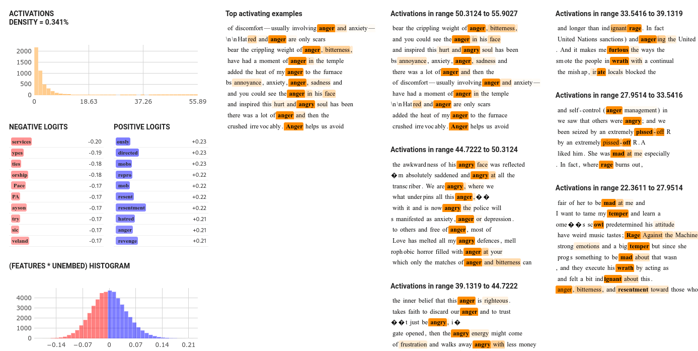
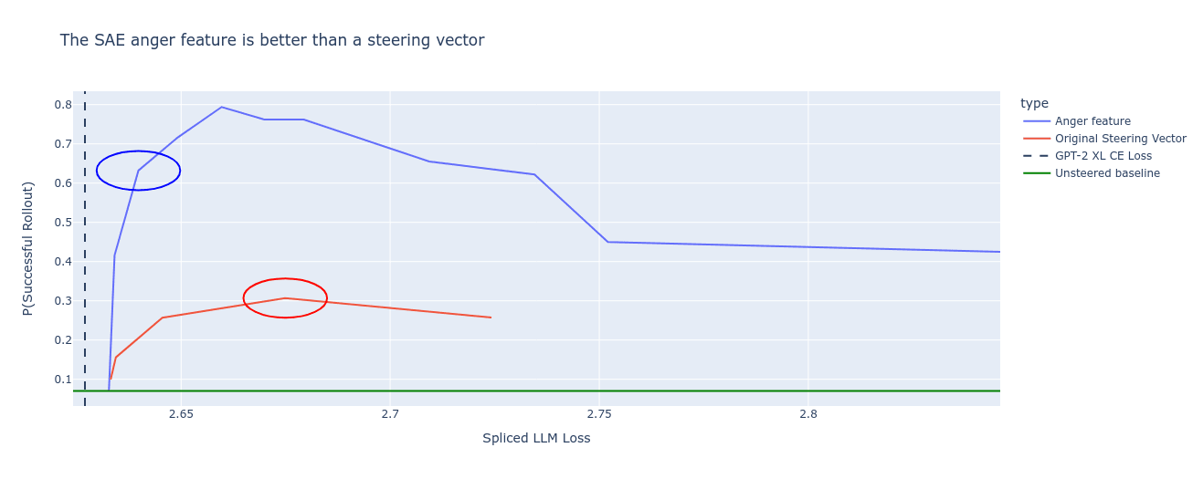
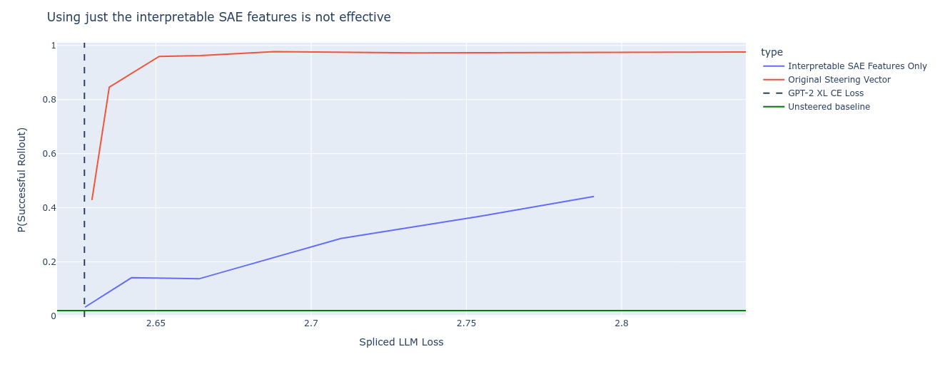
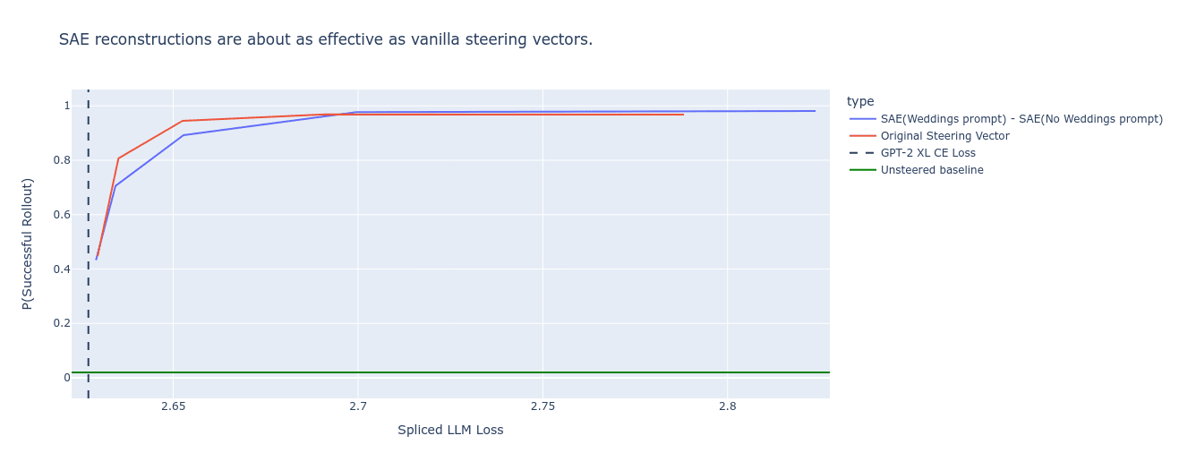
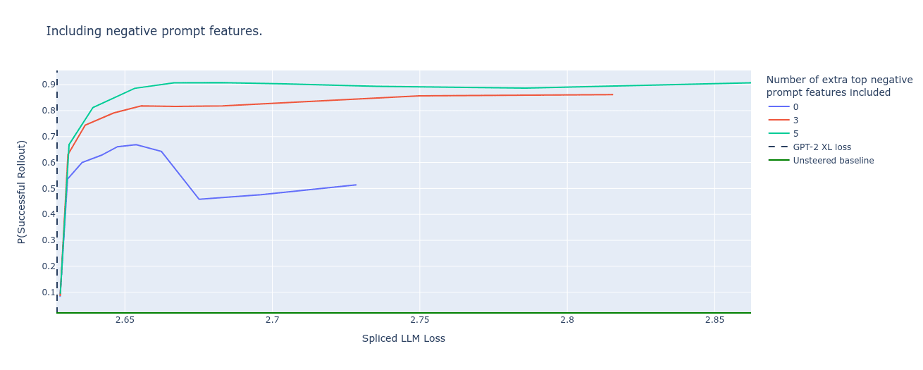
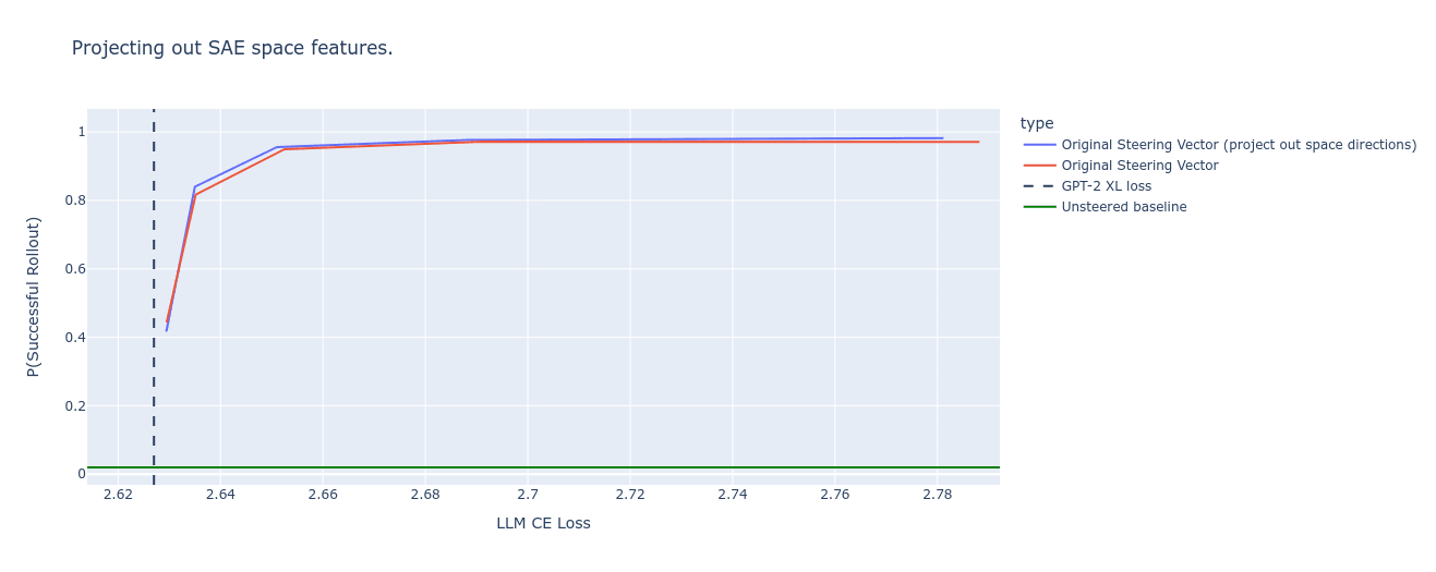 It also removes the double spaces (“| | |”) that can be found in the
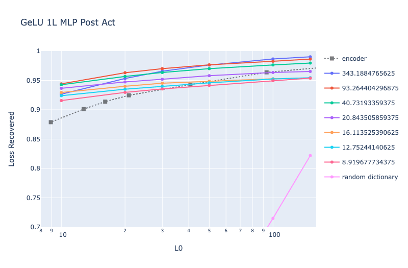
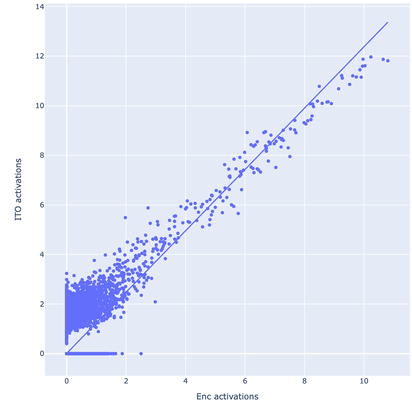
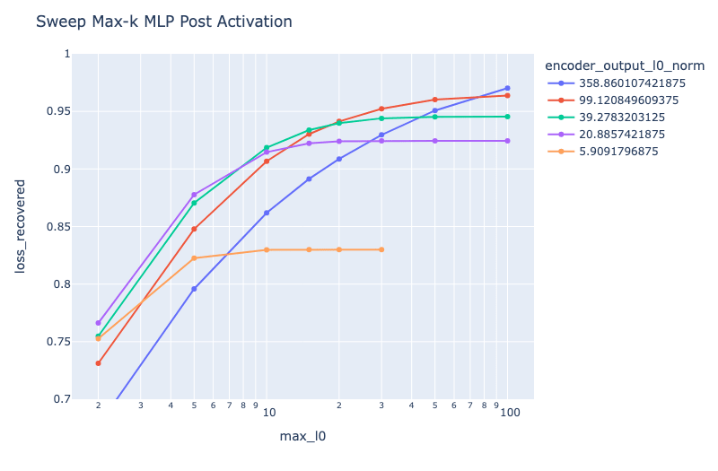
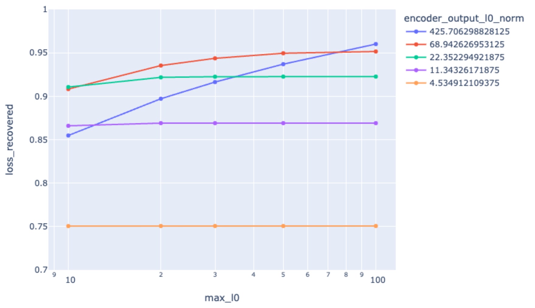
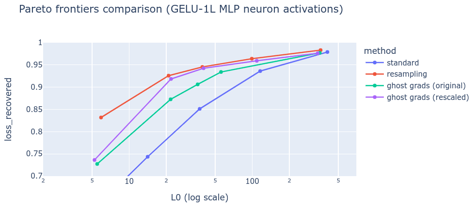
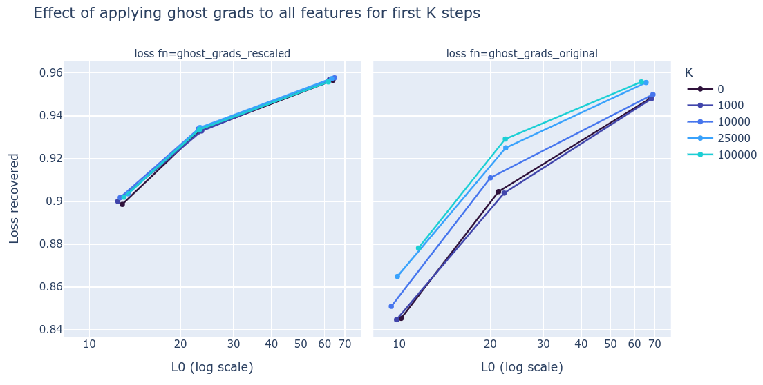
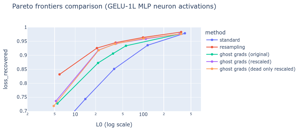
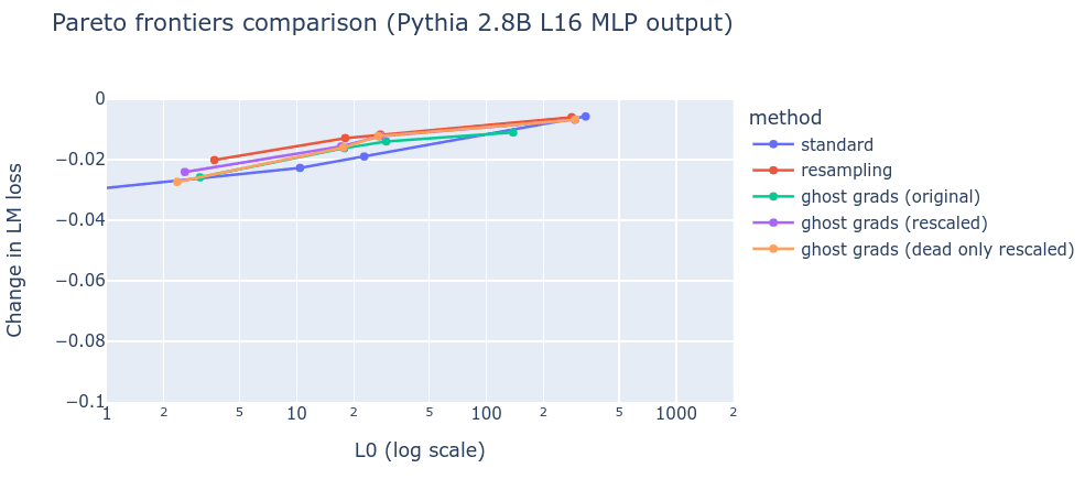
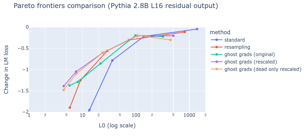
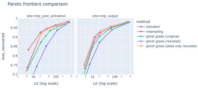
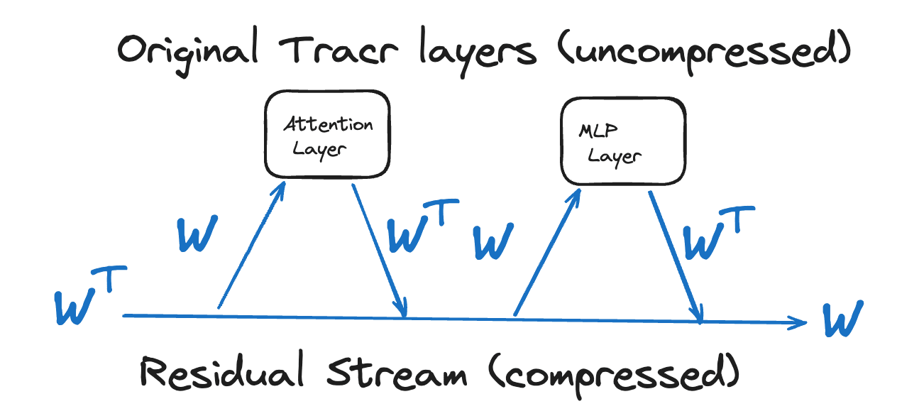
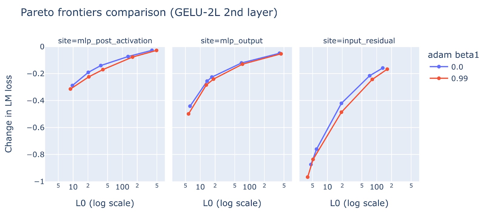
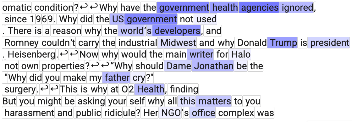
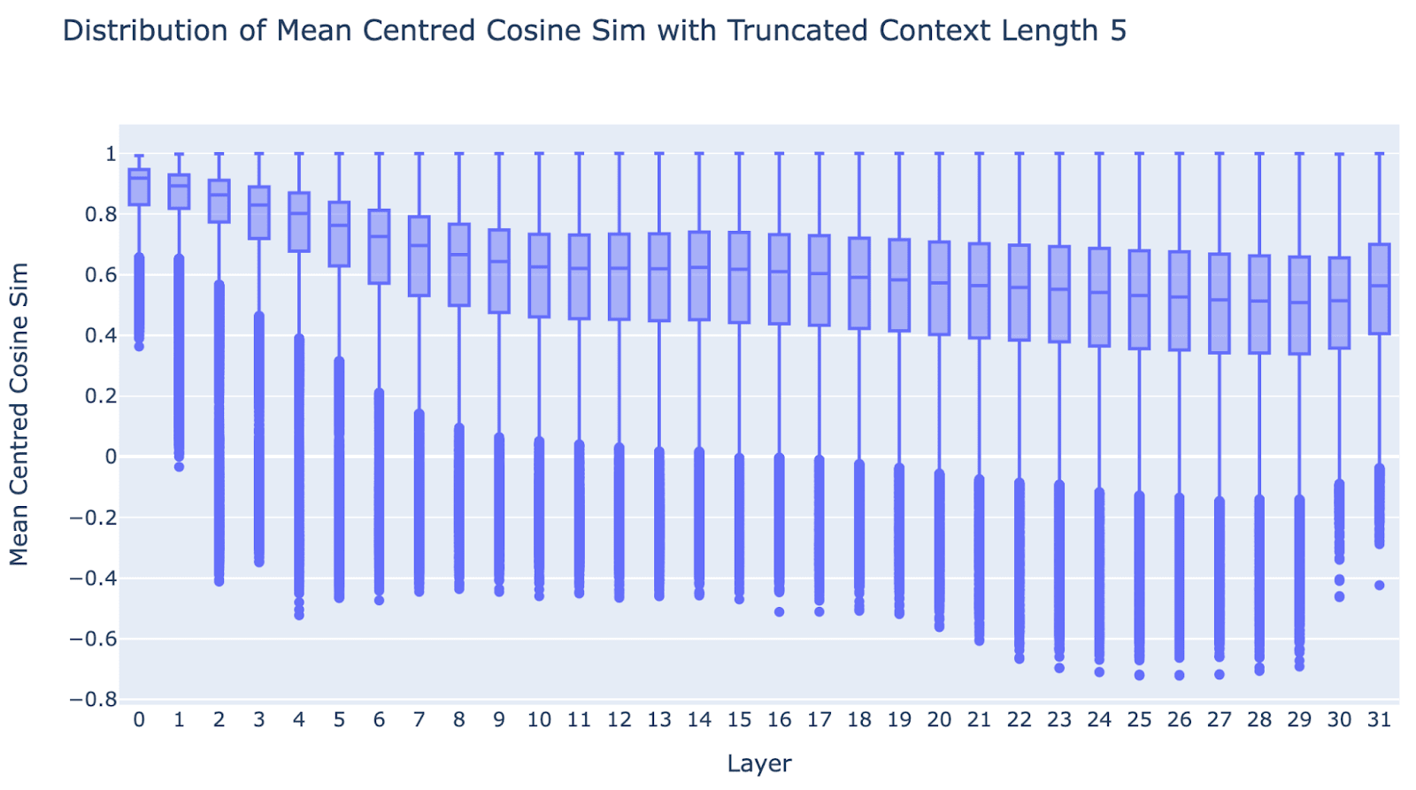
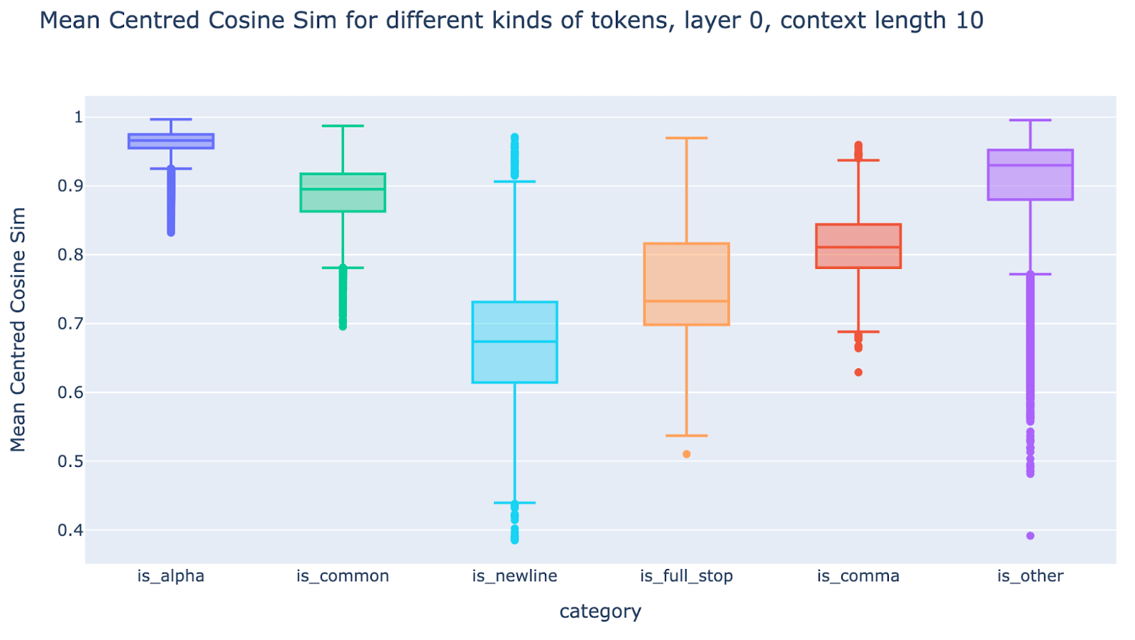

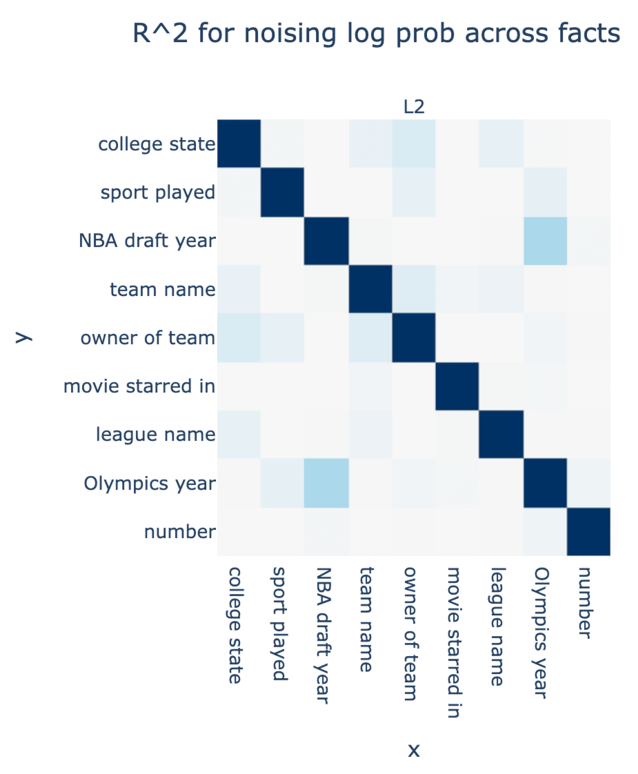
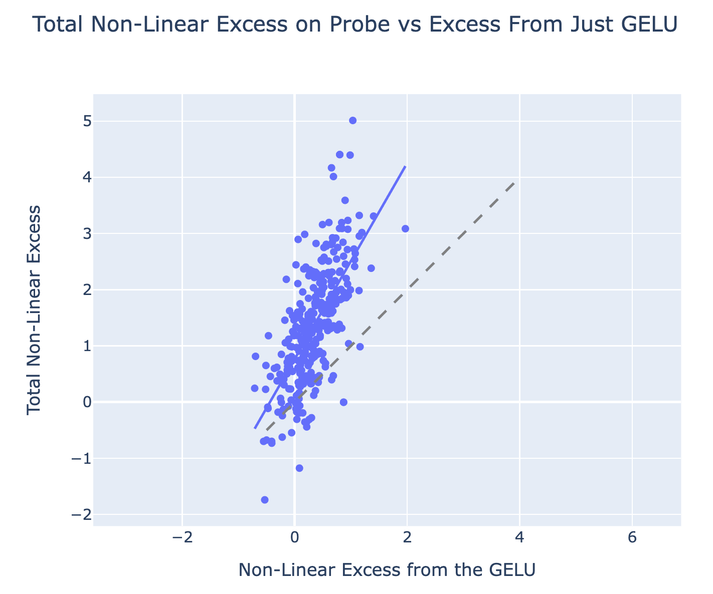
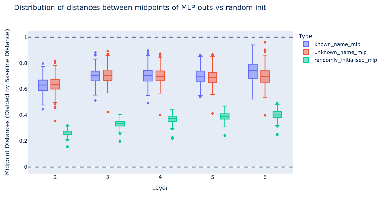

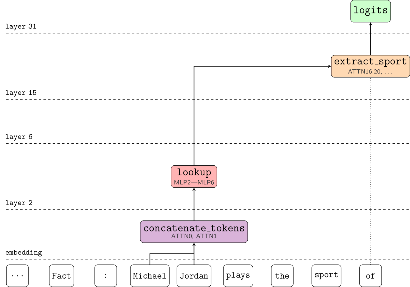
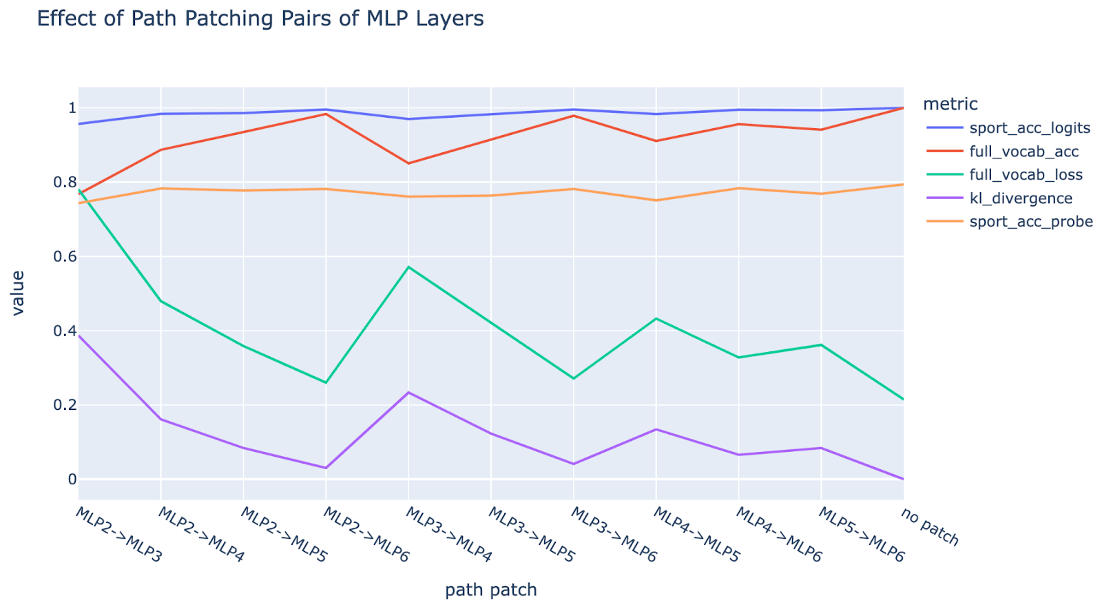
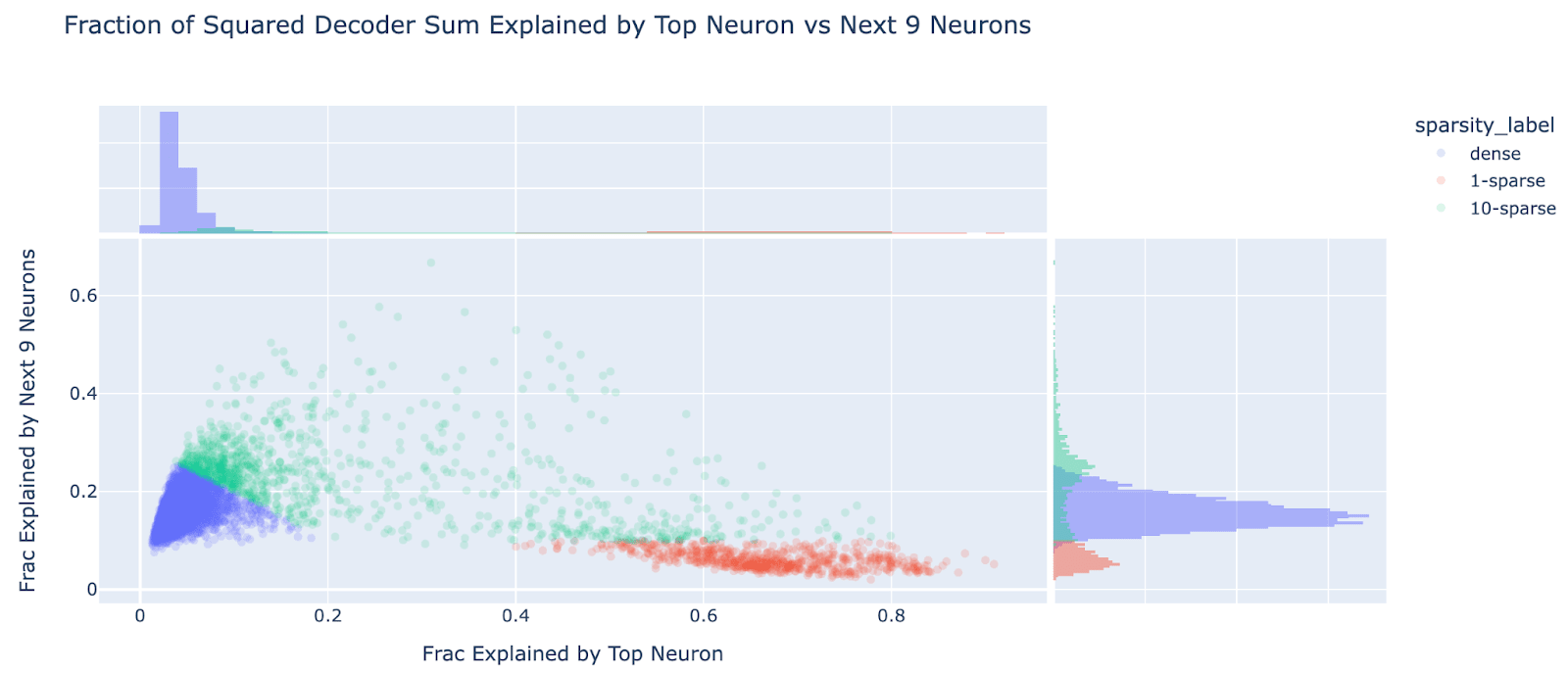
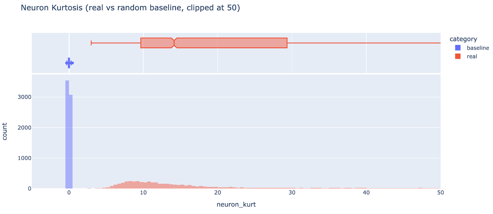
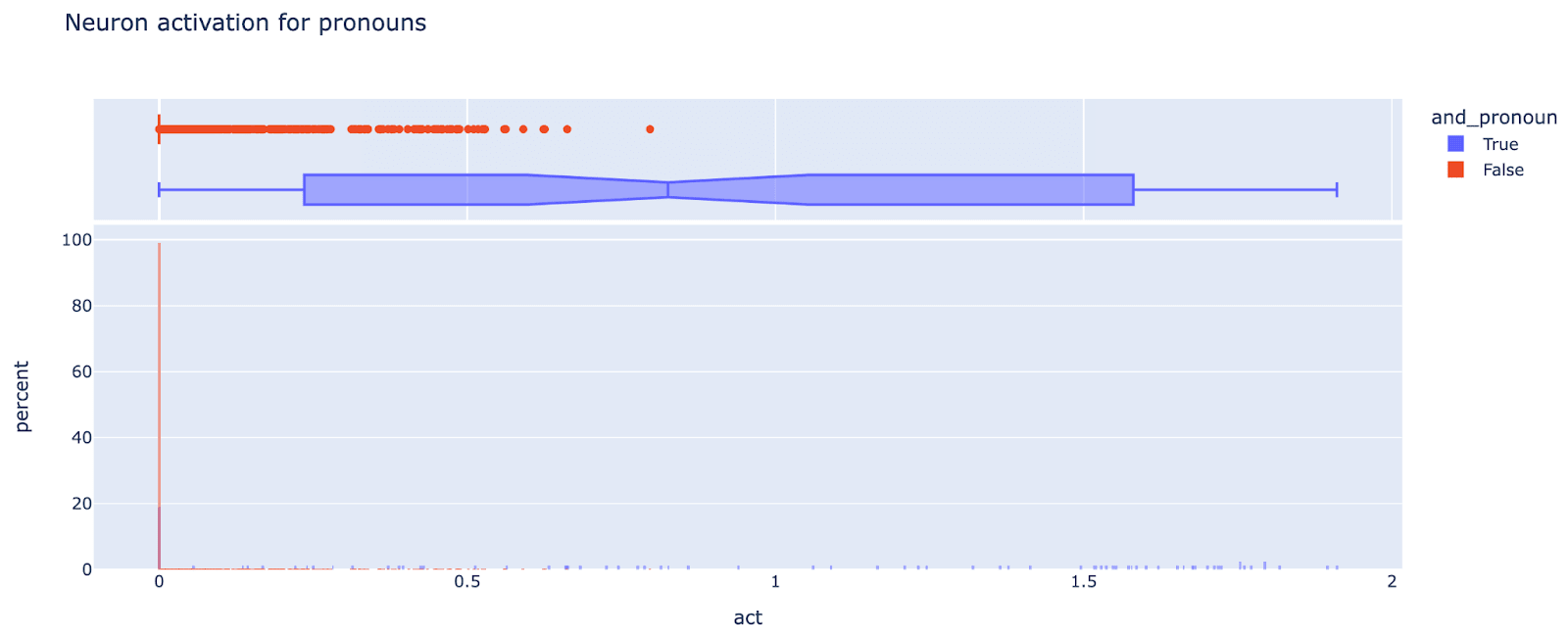
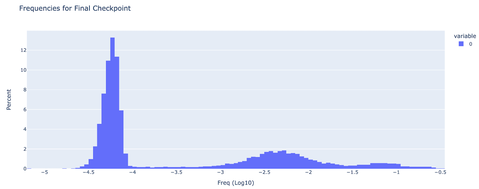
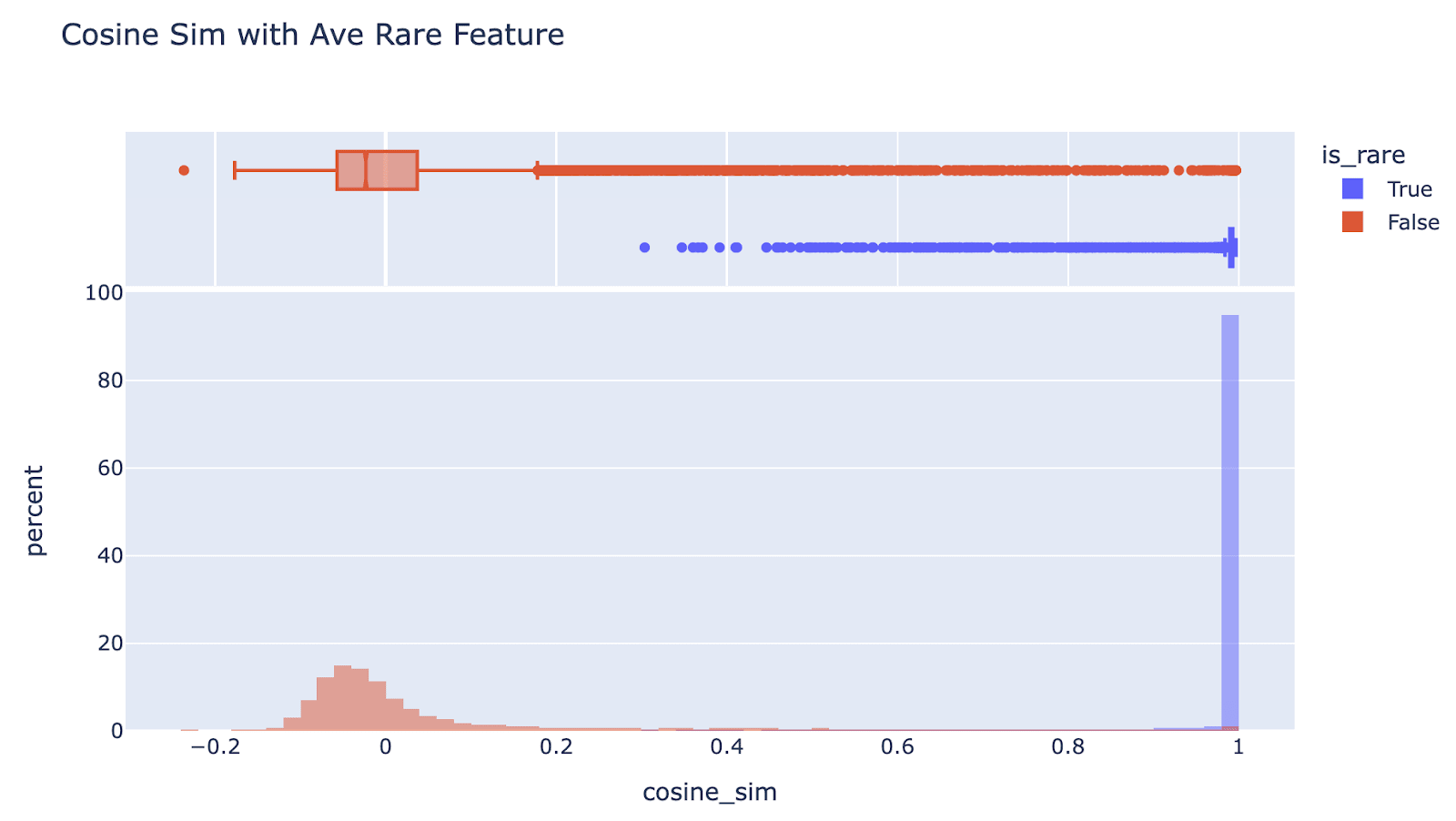
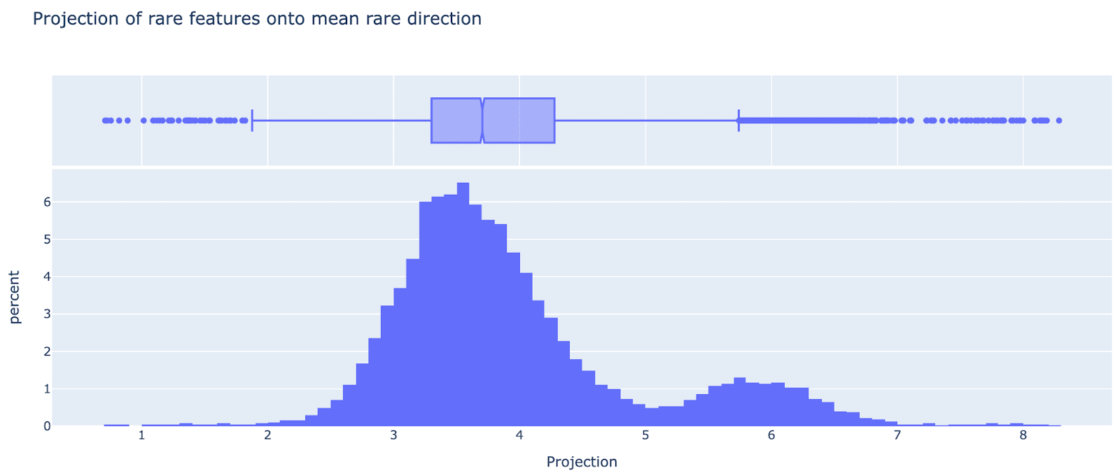
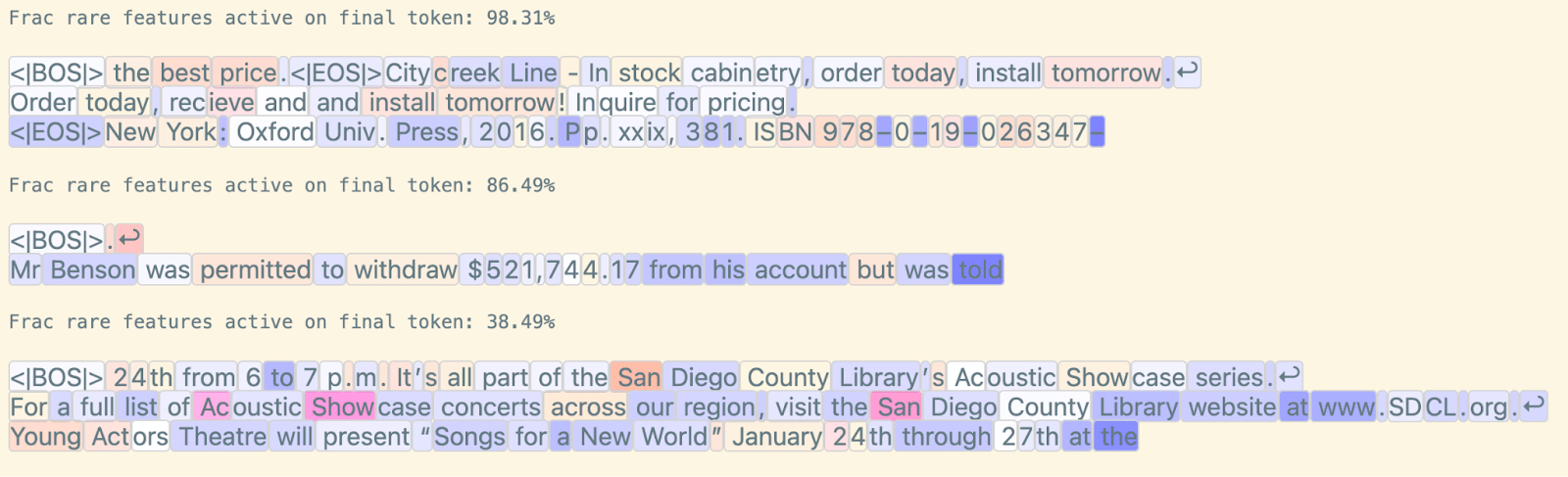
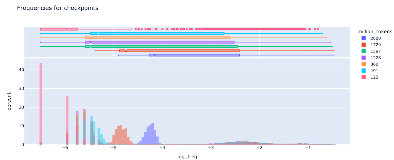
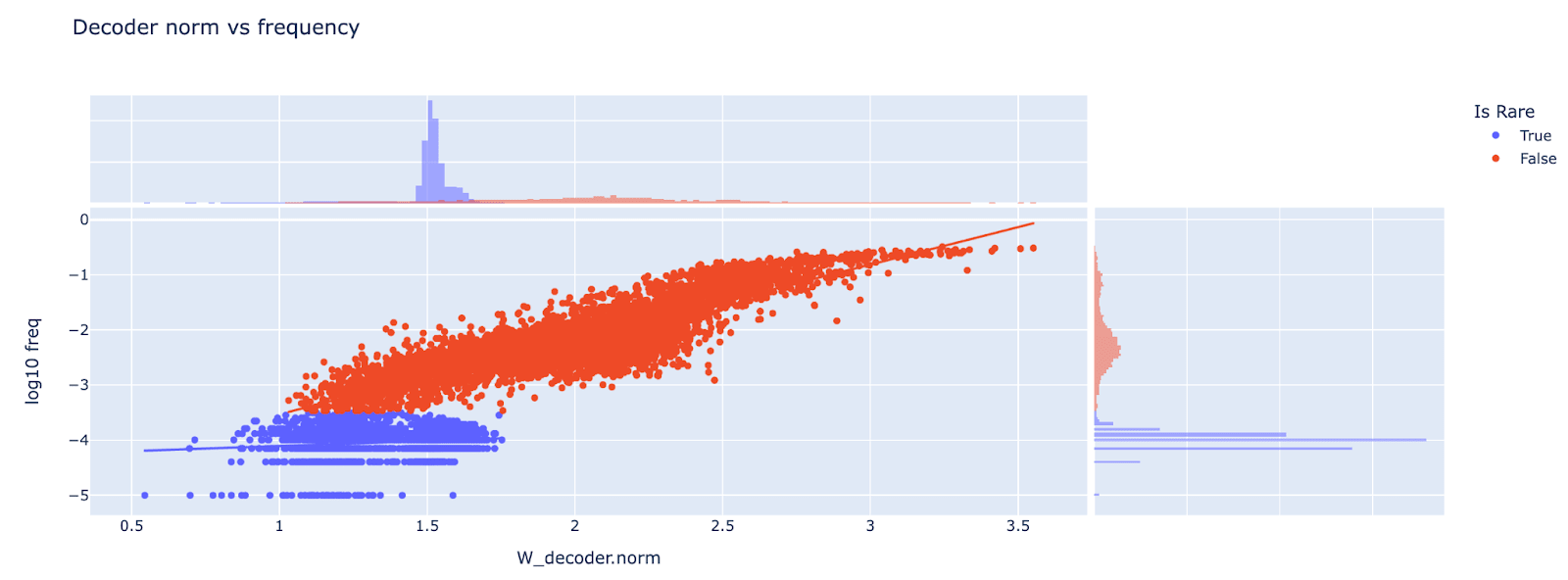
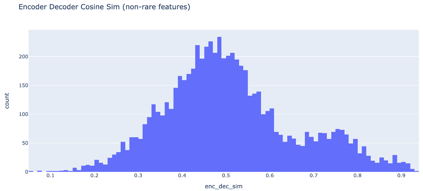
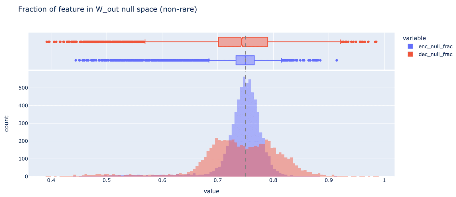
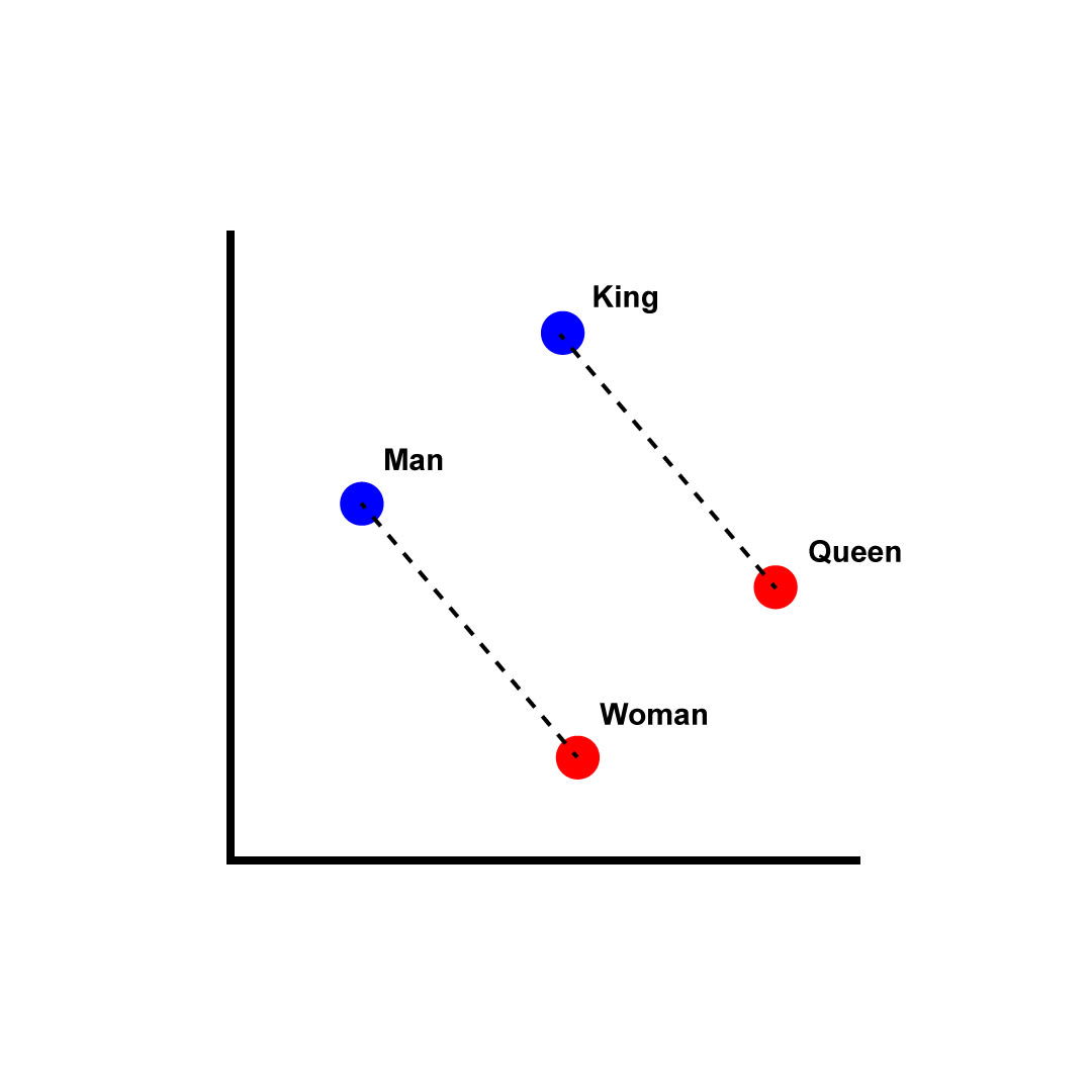


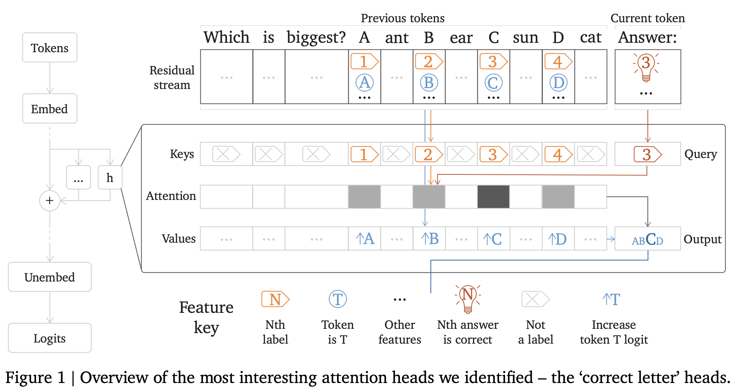
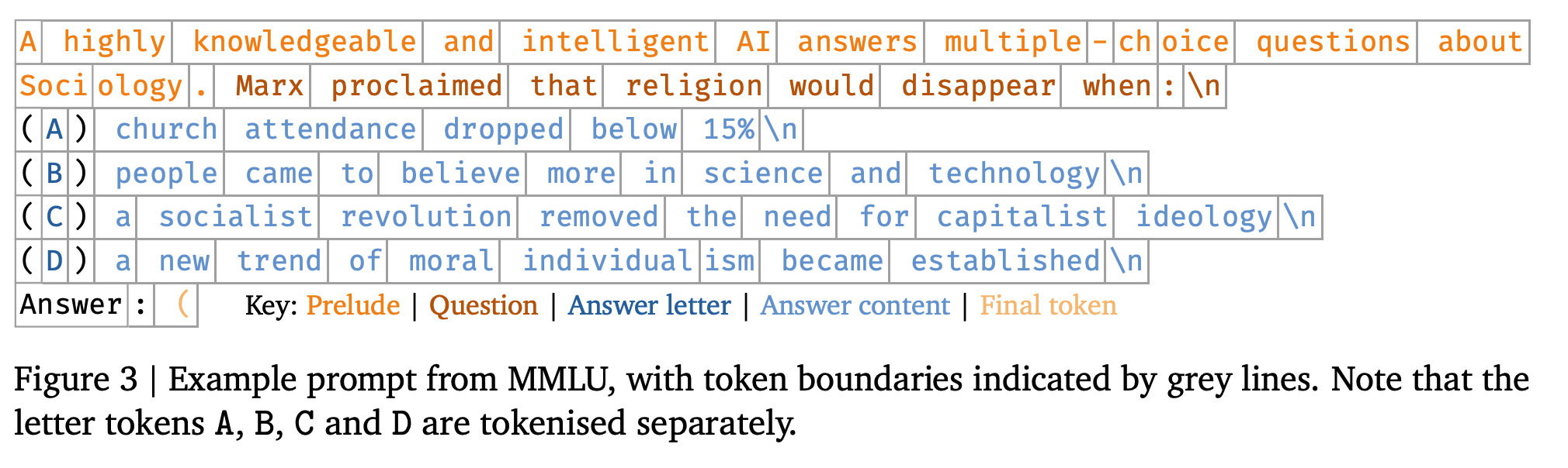
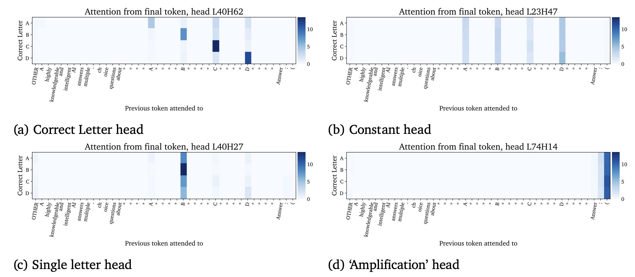
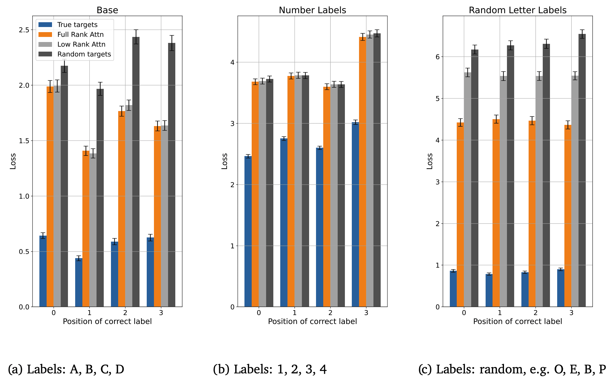
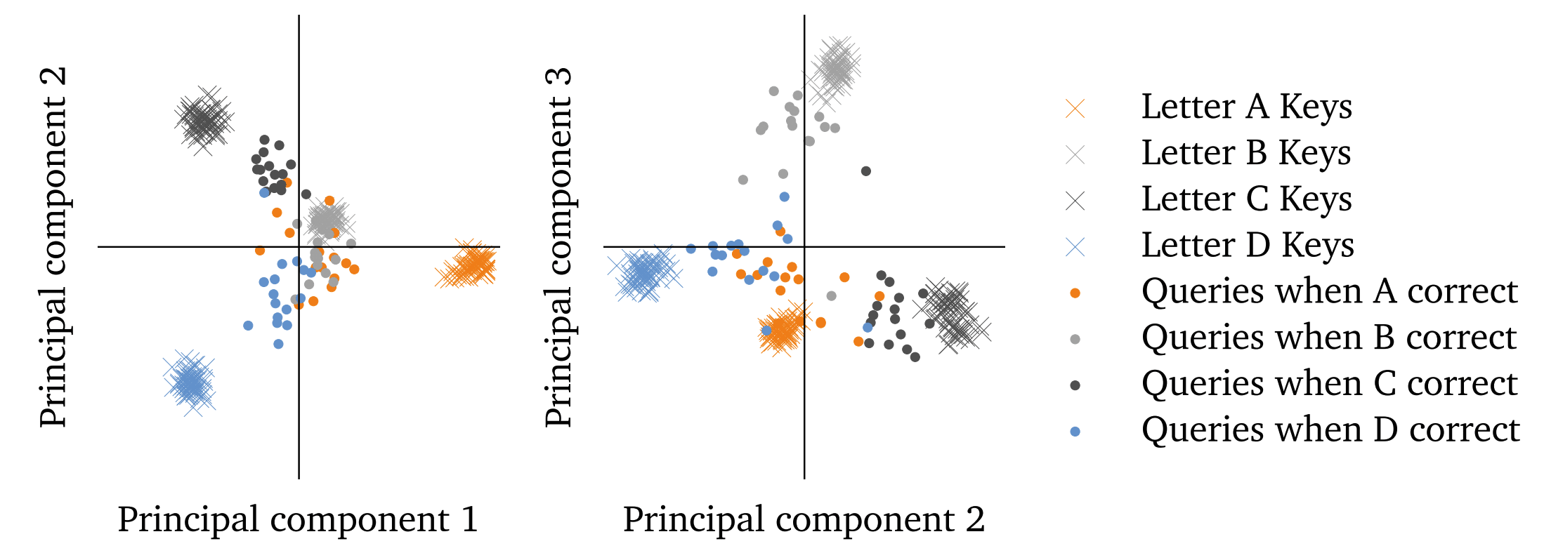
 Tokens are weird, man