Summary. This teaser post sketches our current ideas for dealing with more complex environments. It will ultimately be replaced by one or more longer posts describing these in more detail. Reach out if you would like to collaborate on these issues.

Multi-dimensional aspirations

For real-world tasks that are specified in terms of more than a single evaluation metric, e.g., how much apples to buy and how much money to spend at most, we can generalize Algorithm 2 as follows from aspiration intervals to convex aspiration sets:

• Assume there are d>1 many evaluation metrics ui, combined into a vector-valued evaluation metric u=(u1,…,ud). 
• Preparation: Pick d+1 many linear combinations fj in the space spanned by these metrics so that their convex hull is full-dimensional and contains the origin, and consider the d+1 many policies πj each of which maximizes the expected value of the corresponding function fj. Let Vj(s) and Qj(s,a) be the expected values of u when using πj in state s or after using action a in state s, respectively (see Fig. 1). Let the admissibility simplices V(s) and Q(s,a) be the simplices spanned by the vertices Vj(s) and Qj(s,a), respectively (red and violet triangles in Fig. 1). They replace the feasibility intervals used in Algorithm 2. 
• Policy: Given a convex state-aspiration set E(s)⊆V(s) (central green polyhedron in Fig. 1), compute its midpoint (centre of mass) m and consider the d+1 segments ℓj from m to the corners Vj(s) of V(s) (dashed black lines in Fig. 1). For each of these segments ℓj, let Aj be the (nonempty!) set of actions for which ℓj intersects Q(s,a). For each a∈Aj, compute the action-aspiration E(s,a)⊆Q(s,a) by shifting a copy Cj of E(s) along ℓj towards Vj(s) until the intersection of Cj and ℓj is contained in the intersection of Q(s,a) and ℓj (half-transparent green polyhedra in Fig. 1), and then intersecting Cj with Q(s,a) to give E(s,a) (yellow polyhedra in Fig. 1). Then pick one candidate action from each Aj and randomize between these d+1 actions in proportions so that the corresponding convex combination of the sets E(s,a) is included in E(s). Note that this is always possible because m is in the convex hull of the sets Cj and the shapes of the sets E(s,a) "fit" into E(s) by construction.
• Aspiration propagation: After observing the successor state s′, the action-aspiration E(s,a) is rescaled linearly from Q(s,a) to V(s′) to give the next state-aspiration E(s′), see Fig. 2. 

(We also consider other variants of this general idea) 

Hierarchical decision making

A common way of planning complex tasks is to decompose them into a hierarchy of two or more levels of subtasks. Similar to existing approaches from hierarchical reinforcement learning, we imagine that an AI system can make such hierarchical decisions as depicted in the following diagram (shown for only two hierarchical levels, but obviously generalizable to more levels):

Summary. In this post, we extend the basic algorithm by adding criteria for choosing the two candidate actions the algorithm mixes, and by generalizing the goal from making the expected Total equal a particular value to making it fall into a particular interval. We only use simple illustrative examples of performance and safety criteria and reserve the discussion of more useful criteria for later posts.  

Introduction: using the gained freedom to increase safety

After having introduced the basic structure of our decision algorithms in the last post, in this post we will focus on the core question: How shall we make use of the freedom gained from having aspiration-type goals rather than maximization goals? 

After all, while there is typically only a single policy that maximize some objective function (or very few, more or less equivalent policies), there is typically a much larger set of policies that fulfill some constraints (such as the aspiration to make the expected Total equal some desired value). 

More formally: Let us think of the space of all (probabilistic) policies, Π, as a compact convex subset of a high-dimensional vector space with dimension d≫1 and Lebesgue measure μ. Let us call a policy π∈Π successful iff it fulfills the specified goal, G, and let ΠG⊆Π be the set of successful policies. Then this set has typically zero measure, μ(ΠG)=0, and low dimension, dim(ΠG)≪d, if the goal is a maximization goals, but it has large dimension, dim(ΠG)≈d, for most aspiration-type goals. 

E.g., if the goal is to make expected Total equal an aspiration value, Eτ=E, we typically have dim(ΠG)=d−1 but still μ(ΠG)=0. At the end of this post, we discuss how the set of successful policies can be further enlarged by switching from aspiration values to aspiration intervals to encode goals, which makes the set have full dimension, dim(ΠG)=d, and positive measure, μ(ΠG)>0.

What does that mean? It means we have a lot of freedom to choose the actual policy π∈ΠG that the agent should use to fulfill an aspiration-type goal. We can try to use this freedom to choose policies that promise to be rather safe than unsafe according to some generic safety metric, similar to the impact metrics used in reward function regularization for maximizers.

Depending on the type of goal, we might also want to use this freedom to choose policies that fulfill the goal in a rather desirable than undesirable way according to some goal-related performance metric. 

In this post, we will illustrate this with only very few, "toy" safety metrics, and one rather simple goal-related performance metric, to exemplify how such metrics might be used in our framework. In a later post, we will then discuss more sophisticated and hopefully more useful safety metrics. 

Let us begin with a simple goal-related performance metric since that is the most straightforward.

Simple example of a goal-related performance metric 

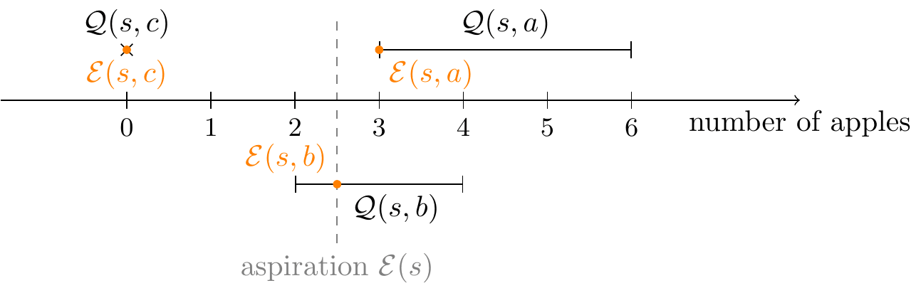
Recall that in step 2 of the basic algorithm, we could make the agent pick any action a− whose action-aspiration is at most as large as the current state-aspiration, E(s,a−)≤E(s), and it can also pick any other action, a+, whose action-aspiration is at least as large as the current state-aspiration, E(s,a+)≥E(s). This flexibility is because in steps 3 and 4 of the algorithm, the agent is still able to randomize between these two actions a−,a+ in a way that makes expected Total, Eτ, become exactly E(s).

If one had an optimization mindset, one might immediately get the idea to not only match the desired expectation for the Total, but also to minimize the variability of the Total, as measured by some suitable statistic such as its variance. In a sequential decision making situation like an MDP, estimating the variance of the Total requires a recursive calculation that anticipates future actions, which can be done but is not trivial. We reserve this for a later post.

Let us instead look at a simpler metric to illustrate the basic approach: the (relative, one-step) squared deviation of aspiration, which is very easy to compute:

The rationale for this is that at any time, the action aspirations E(s,a±) are the expected values of Total-to-go conditional on taking action a±, so keeping them close to E(s) will tend to lead to a smaller variance. Indeed, that variance is lower bounded by (E(s,a−)−E(s))2:p:(E(s,a+)−E(s))2, where p is the probability for choosing a+ calculated in step 3 of Algorithm 1.  

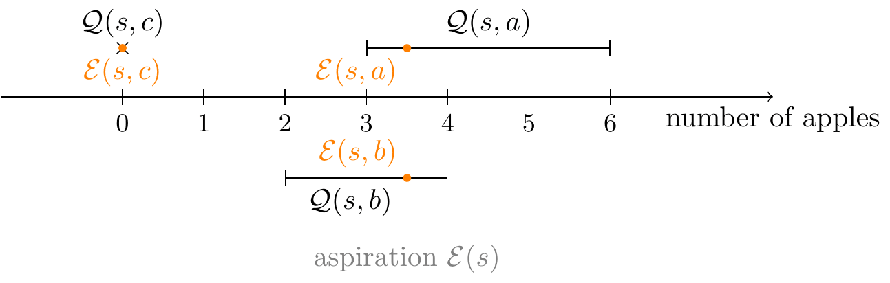
If the action space is rich enough, there will often be at least one action the action-aspiration of which equals the state-aspiration, E(s,a)=E(s), because the state-aspiration is contained in that action's feasibility interval, E(s)∈Q(s,a). There might even be a large number of such actions. This will in particular be the case in the early steps of an episode. This is because often one can distribute the amount of effort spent on a task more or less flexibly over time; as long as there is enough time left, one might start by exerting little effort and then make up for this in later steps, or begin with a lot of effort and then relax later. 

If this is the case, then minimizing SDA(s,a) simply means choosing one of the actions for which E(s)∈Q(s,a) and thus E(s,a)=E(s) and thus SDA(s,a)=0, and then put a−=a+=a. When there are many such candidate actions a, that will still leave us with some remaining freedom for incorporating some other safety criteria to choose between them, maybe deterministically. One might thus think that this form of optimization is safe enough and should be performed because it gets rid of all variability and randomization in that step. 

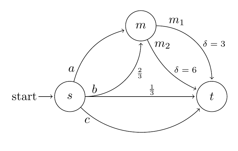
For example: Assume the goal is to get back home with fourteen apples within a week, and the agent can harvest or eat at most six apples on each day (apples are really scarce). Then each day the agent might choose to harvest or eat any number of apples, as long as its current stock of apples does not deviate from fourteen by more than six times the remaining number of days. Only in the last several days it might then have to harvest or eat exactly six apples per day, to make up for earlier deviations and to land at fourteen apples sharp eventually.   

But there's at least two objections to minimizing SDA. First, generically, we can not be sure enough that there will indeed be many different actions for which E(s)∈Q(s,a), and so restricting our choice to the potentially only few actions that fulfill this might not allow us to incorporate safety criteria to a sufficient level. In particular, we should expect that the latter is often the case in the final steps of an episode, where there might at best be a single such action that perfectly makes up for the earlier under- or over-achievements, or even no such action at all. Second, getting rid of all randomization goes against the intuition of some many members of our project team that randomization is a desirable feature that tends to increase rather than decrease safety (this intuition also underlies the alternative approach of quantilization). 

We think that one should thus not minimize performance metrics such as SDA or any other of the later discussed metrics, but at best use them as soft criteria. Arguably the most standard way to do this is to use a softmin (Boltzmann) policy for drawing both candidate actions a− and a+ independently of each other, on the basis of their SDA (or another metric's) scores: 

restricted to those a−,a+ with Q(s,a−)≤Q(s)≤Q(s,a+), and for some sufficiently small inverse temperature β>0 to ensure sufficient randomization. 

While the SDA criterion is about keeping the variance of the Total rather low and is thus about fulfilling the goal in a presumably more desirable way from the viewpoint of the goal-setting client, the more important type of action selection criterion is not goal- but safety-related. So let us now look at the latter type of criterion. 

Toy example of a generic safety metric

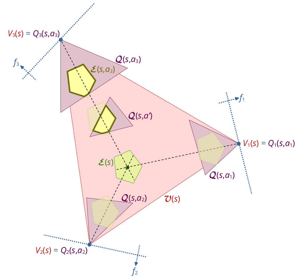
As the apple example above shows, the agent might easily get into a situation where it seems to be a good idea to take an extreme action. A very coarse but straightforward and cheap to compute heuristic for detecting at least some forms of extreme actions is when the corresponding aspiration is close to an extreme value of the feasibility interval: E(s,a)≈Q––(s,a) or E(s,a)≈¯¯¯¯Q(s,a). 

This motivates the following generic safety criterion, the (relative, one-step) squared extremity of aspiration:

(The factor 4 is for normalization only) 

The rationale is that using actions a−,a+ with rather low values of SEA would tend to make the agent's aspirations stay close to the center of the relevant feasibility intervals, and thus hopefully also make its actions remain moderate in terms of the achieved Total. 

Let's see whether that hope is justified by studying what minimizing SEA would lead to in the above apple example:

• On day zero, E(s0)=14, V(s)=[−42,42], and Q(s0,a)=[a−36,a+36] for a∈{−6,…,6}. Since the current state-aspiration, 14, is in all actions' feasibility intervals, all action-aspirations are also 14. Both the under- and overachieving action with smallest SEA is thus a−=a+=6, since this action's Q-midpoint, 6, is closest to its action-aspiration, 14. The corresponding λ=−30∖14∖42=44/72. 
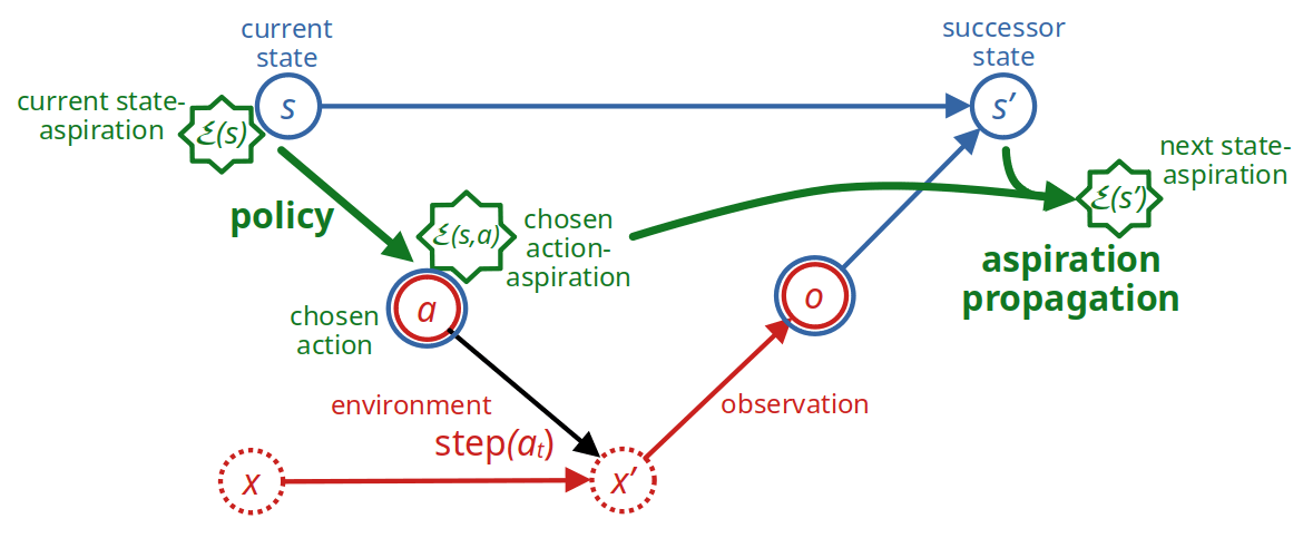
• On the next day, the new feasibility interval is V(s1)=[−36,36], so the new state-aspiration is E(s1)=−36:44/72:36=8. This is simply the difference between the previous state-aspiration, 14, and the received Delta, 6. (It is easy to see that the aspiration propagation mechanism used has this property whenever the environment is deterministic). Since Q(s1,a)=[a−30,a+30]∋8, we again have E(s1,a)=8 for all a, and thus again a−=a+=6 since 6 is closest to 8. 
• On the next day, E(s2)=8−6=2,  Q(s2,a)=[a−24,a+24]∋2, and now a−=a+=2 since 2 is closest to 2. Afterwards, the agent neither harvests not eats any apples but lies in the grass, relaxing.

The example shows that the consequence of minimizing SEA is not, as hoped, always an avoidance of extreme actions. Rather, the agent chooses the maximum action in the first two steps (which might or might not be what we eventually consider safe, but is certainly not what we hoped the criterion would prevent). 

Maybe we should compare Deltas rather than aspirations if we want to avoid this? So what about (relative, one-step) squared extremity of Delta,  

If the agent minimizes this instead of SEA in the apple example, it will procrastinate by choosing a−=a+=0 for the first several days, as long as 14∈Q(st,0)=[6t−36,36−6t]. This happens on the first four days. On the fifth day (t=4), it will still have aspiration 14. It will then again put a−=0 with action-aspirationE(s4,0)=12=¯¯¯¯Q(s4,0), but it will put a+=2 with action-aspiration E(s4,2)=14. Since the latter equals the state-aspiration, the calculated probability in step 3 of the algorithm turns out to be p=1, meaning the agent will use action a+ for sure after all, rather than randomizing it with a−. This leaves an aspiration of 14−2=12. On the remaining two days, the agent then has to use a=6 to fulfill the aspiration in expectation.

Huh? Even though both heuristics seem to be based on a similar idea, one of them leads to early extreme action and later relaxation, and the other to procrastination and later extreme action, just the opposite. Neither of them avoids extreme actions. 

One might think that one could fix the problem by simply adding the two metrics up into a combined safety loss, 

But in the apple example, the agent would still harvest six apples on the first day, since (14−6)2+(6−0)2<(14−5)2+(5−0)2. Only on the second day, it would harvest just four instead of six apples, because (8−4)2+(4−0)2 is minimal. On the third day: two apples because (4−2)2−(2−0)2 is minimal. Then one apple, and then randomize between one or zero apples, until it has the 14 apples, or until the last day has come where it needs to harvest one last apple.

The main reason for all these heuristics failing in that example is their one-step nature which does not anticipate later actions. In a later post we will thus study more complex, farsighted metrics that can still be computed efficiently in a recursive manner, such as disordering potential,

which measures the largest Shannon entropy in the state trajectory that the agent could cause if it aimed to, or terminal state distance,

which measures the expected distance between the terminal and initial state according to some metric d on state space and depends on the actual policy π and aspiration propagation scheme E(s)→E(s,a)→E(s′) that the agent uses. 

But before looking at such metrics more closely, let us finish this post by discussing other ways to combine several performance and/or safety metrics. 

Using several safety and performance metrics

Defining a combined loss function like L(s,a) above by adding up components is clearly not the only way to combine several safety and/or performance metrics, and is maybe not the best way to do that because it allows unlimited trade-offs between the components. 

It also requires them to be measured in the same units and to be of similar scale, or to make them so by multiplying them with suitable prefactors that would have to be justified. This at least can always be achieved by some form of normalization, like we did above to make SEA and SED dimensionless and bounded by [0,1].

Trade-offs between several normalized loss components Li(s,a)∈[0,1] can be limited in all kinds of ways, for example by using some form of economics-inspired "safety production function" such as the CES-type function 

with suitable parameters ρ and bi>0 with ∑ibi=1. For ρ=1, we just have a linear combination that allows for unlimited trade-offs. At the other extreme, in the limit of ρ→−∞, we get L(s,a)=maxiLi(s,a), which does not allow for any trade-offs.

Such a combined loss function can then be used to determine the two actions a−,a+, e.g., using a softmin policy as suggested above. 

An alternative to this approach is to use some kind of filtering approach to prevent unwanted trade-offs. E.g., one could use one of the safety loss metrics, L1(s,a), to restrict the set of candidate actions to those with sufficiently small loss, say withL1(s,a)≤mina′L1(s,a′):0.1:maxa′L1(s,a′), then use a second metric, L2, to filter further, and so on, and finally use the last metric, Lk, in a softmin policy.

As we will see in a later post, one can come up with many plausible generic safety criteria, and one might be tempted to just combine them all in one of these ways, in the hope to thereby have found the ultimate safety loss function or filtering scheme. But it might also well be that one will have forgotten some safety aspects and end up with an imperfect combined safety metric. This would be just another example of a misspecified objective function. Hence we should again resist falling into the optimization trap of strictly minimizing that combined loss function, or the final loss function of the filtering scheme. Rather, the agent should probably still use a sufficient amount of randomization in the end, for example by using a softmin policy with sufficient temperature. 

If it is unclear what a sufficient temperature is, one can set the temperature automatically so that the odds ratio between the least and most likely actions equals a specified value: β:=η/(maxaL(s,a)−minaL(s,a)) for some fixed η>0.

More freedom via aspiration intervals

We saw earlier that if the goal is to make expected Total equal an aspiration value, Eτ=E∈R, the set of successful policies has large but not full dimension and thus still has measure zero. In other words, making expected Total exactly equal to some value still requires policies that are very "precise" and in this regard very "special" and potentially dangerous. So we should probably allow some leeway, which should not make any difference in almost all real-world tasks but increase safety further by avoiding solutions that are too special. 

Of course the simplest way to provide this leeway would be to just get rid of the hard constraint altogether and replace it by a soft incentive to make Eτ close to E∈R, for example by using a softmin policy based on the mean squared error. This might be acceptable for some tasks but less so for others. The situation appears to be somewhat similar to the question of choosing estimators in statistics (e.g., a suitable estimator of variance), where sometimes one only wants the estimator with the smallest standard error, not caring for bias (and thus not having any guarantee about the expected value), sometimes one wants an unbiased estimator (i.e., an estimator that comes with an exact guarantee about the expected value), and sometimes one wants at least a consistent estimator that is unbiased in the limit of large data and only approximately unbiased otherwise (i.e., have only an asymptotic rather than an exact guarantee about the expected value). 

For tasks where one wants at least some guarantee about the expected Total, one can replace the aspiration value by an aspiration interval E=[e–,¯¯¯e]⊆R and require that Eτ∈E. 

The basic algorithm (algorithm 1) can easily be generalized to this case and only becomes a little bit more complicated due to the involved interval arithmetic:

Decision algorithm 2    

Similar to algorithm 1, we... 

• set action-aspiration intervals E(s,a)=[e–(s,a),¯¯¯e(s,a)]⊆Q(s,a) for each possible action a∈A on the basis of the current state-aspiration interval E(s)=[e–(s),¯¯¯e(s)] and the action's feasibility interval Q(s,a), trying to keep E(s,a) similar to and no wider than E(s),
• choose an "under-achieving" action a− and an "over-achieving" action a+ w.r.t. the midpoints of the intervals E(s) and E(s,a),
• choose probabilistically between a− and a+ with suitable probabilities, and
• propagate the action-aspiration interval E(s,a) to the new state-aspiration interval E(s′) by rescaling between the feasibility intervals of a and s′.

More precisely: Let m(I) denote the midpoint of interval I. Given state s and state-aspiration interval E(s),

1. For all a∈A, let E(s,a) be the closest interval to E(s) that lies within Q(s,a) and is as wide as the smaller of E(s) and Q(s,a).
2. Pick some a−,a+∈A with m(E(s,a−))≤m(E(s))≤m(E(s,a+))
3. Compute p←m(E(s,a−))∖m(E(s))∖m(E(s,a−))
4. With probability p, put a←a+, otherwise put a←a−
5. Implement action a in the environment and observe successor state s′←step(s,a)
6. Compute λ––←Q––(s,a)∖e–(s,a)∖¯¯¯¯Q(s,a) and e–(s′)←V––(s′):λ––:¯¯¯¯V(s′), and similarly for ¯¯¯λ and ¯¯¯e(s′)

Note that the condition that no E(s,a) must be wider than E(s) in step 1 ensures that, independently of what the value of p computed in step 3 will turn out to be, any convex combination q−:p:q+ of values q±∈E(s,a±) is an element of E(s). This is the crucial feature that ensures that aspirations will be met:

Theorem (Interval guarantee)

If the world model predicts state transition probabilities correctly and the episode-aspiration interval E(s0) is a subset of the initial state's feasibility interval, E(s0)⊆V(s0), then algorithm 2 fulfills the goal Eτ∈E(s0).

The Proof is completely analogous to the proof in the last post, except that each occurrence of V(s,e)=E(s)∈V(s) and Q(s,a,e)=E(s,a)∈Q(s,a) is replaced by V(s,e)∈E(s)⊆V(s) and Q(s,a,e)∈E(s,a)⊆Q(s,a), linear combination of sets is defined as cX+c′X′={cx+c′x′:x∈X,x′∈X′}, and we use the fact that m(E(s,a−)):p:m(E(s,a+))=m(E(s)) implies E(s,a−):p:E(s,a+)⊆E(s).

Special cases

Satisficing. The special case where the upper end of the aspiration interval coincides with the upper end of the feasibility interval leads to a form of satisficing guided by additional criteria.

Probability of ending in a desirable state. A subcase of satisficing is when all Deltas are 0 except for some terminal states where it is 1, indicating that a "desirable" terminal state has been reached. In that case, the lower bound of the aspiration interval is simply the minimum acceptable probability of ending in a desirable state.

Before discussing some more interesting safety metrics, we will first introduce in the next post a few simple environments to test these criteria in...

Summary. In this post, we present the formal framework we adopt during the sequence, and the simplest form of the type of aspiration-based algorithms we study. We do this for a simple form of aspiration-type goals: making the expectation of some variable equal to some given target value. The algorithm is based on the idea of propagating aspirations along time, and we prove that the algorithm gives a performance guarantee if the goal is feasible. Later posts discuss safety criteria, other types of goals, and variants of the basic algorithm.

Assumptions

In line with the working hypotheses stated in the previous post, we assume more specifically the following in this post:

• The agent is a general-purpose AI system that is given a potentially long sequence of tasks, one by one, which it does not know in advance. Most aspects of what we discuss focus on the current task only, but some aspects relate to the fact that there will be further, unknown tasks later (e.g., the question of how much power the agent shall aim to retain at the end of the task).
• It possesses an overall world model that represents a good enough general understanding of how the world works.
• Whenever the agent is given a task, an episode begins and its overall world model provides it with a (potentially much simpler) task-specific world model that represents everything that is relevant for the time period until the agent gets a different task or is deactivated, and that can be used to predict the potentially stochastic consequences of taking certain actions in certain world states.
• That task-specific world model has the form of a (fully observed) Markov Decision Process (MDP) that however does not contain a reward function R but instead contains what we call an evaluation function related to the task (see 2nd to next bullet point).
• As a consequence of a state transition, i.e., of taking a certain action a in a certain state s and finding itself in a certain successor state s′, a certain task-relevant evaluation metric changes by some amount. Importantly, we do not assume that the evaluation metric inherently encodes things of which more is better. E.g., the evaluation metric could be global mean temperature, client's body mass, x coordinate of the agent's right thumb, etc. We call the step-wise change in the evaluation metric the received Delta in that time step, denoted δ. We call its cumulative sum over all time steps of the episode the Total, denoted τ. Formally, Delta and Total play a similar role for our aspiration-based approach as the concepts of "reward" and "return" play for maximization-based approaches. The crucial difference is that our agent is not tasked to maximize Total (since the evaluation metric does not have the interpretation of "more is better") but to aim for some specific value of the Total.
• The evaluation function contained in the MDP specifies the expected value of δ for all possible transitions: Eδ(s,a,s′).^[1]

First challenge: guaranteeing the fulfillment of expectation-type goals

The challenge in this post is to design a decision algorithm for tasks where the agent's goal is to make the expected (!) Total equal (!) a certain value E∈R which we call the aspiration value. ^[2] This is a crucial difference from a "satisficing" approach that would aim to make expected Total at least as large as E and would thus still be happy to maximize Total. Later we consider other types of tasks, both less restrictive ones (including those related to satisficing) and more specific ones that also care about other aspects of the resulting distribution of Total or states.

It turns out that we can guarantee the fulfillment of this type of goal under some weak conditions!

Notice that a special case of such expectation-type goals is making sure that the probability of reaching a certain set of acceptable terminal states equals a certain value, because we can simply assume that each such acceptable terminal state gives 1 Delta and all others give zero Delta. We will come back to that special case in the next post when discussing aspiration intervals.

Example: Shopping for apples

• The agent is a certain household's AI butler. Among all kinds of other tasks, roughly once a week it is tasked to go shopping for apples. When it gets this task in the morning, an apple shopping episode begins, which ends when the agent returns to the household to get new instructions or is called by a household member on its smartphone, or when its battery runs empty.
• The relevant evaluation metric for this task is the household's and agent's joint stock of apples. It changes by some Delta each time the agent gets handed some apples by a merchant or takes some from the supermarket's shelf or when some apples fall from its clumsy hands or get stolen by some robot hater (or when some member of the household eats an apple).
• As the household's demand for apples is 21 apples per week on average, the task in a single apple shopping episode is to buy a certain number E of apples in expectation. They also want to maintain some small stock for hard times, say about 5 apples. So the household's policy is to set the aspiration to E=21+(5−x), where x is its current stock of apples. As this is a recurrent task, it is perfectly fine if this aspiration is only fulfilled in expectation if the Total doesn't vary too much, since over many weeks (and assuming long-lived apples), the deviations will probably average out and the stock will vary around 26 apples right after a shopping mission and 5 apples just before the next shopping mission. In reality, the household would of course also want the variance to be small, but that is a performance criterion we will only add later.

Possible generalizations (can be skipped safely)

In later posts, we will generalize the above assumptions in the following ways:

• Instead of as a single value E∈R that expected Total shall equal, the task can be given as an aspiration interval E=[e–,¯¯¯e] into which expected Total shall fall (e.g., "buy about 21+(5−x)±2 apples").
• Instead of a single evaluation metric (stock of apples), there can be d>1 many evaluation metrics (stock of apples, stock of pears, and money in pocket), and the task can be given as a convex aspiration set E⊆Rd (e.g., buy at least two apples and one pear but don't spend more than 1 Euro per item).
• Instead of in terms of evaluation metrics, the task could be given in terms of the terminal state of the episode, by specifying a particular "desired" state, a set of "acceptable" states, a desired probability distribution of terminal states, or a set of acceptable probability distribution of terminal states. For example, demanding that the expected number of stocked apples after the episode be 26 is the same as saying that all probability distributions of terminal states are acceptable that have the feature that the expected number of stocked apples is 26. A more demanding task would then be to say that only those probability distributions of terminal states are acceptable for which the expected number of stocked apples is 26, its standard deviation is at most 3, its 5 per cent quantile is at least 10, and the 5 per cent quantile of the number of surviving humans is at least 8 billion.
• The world model might have a more general form than an MDP: to represent different forms of uncertainty, it might be an only partially observed MDP (POMDP), or an ambiguous POMDP (APOMDP); to represent complex tasks, it might be a hierarchical MDP whose top-level actions (e.g., buy 6 apples from this merchant) are represented as lower-level MDPs with lower-level aspirations specified in terms of auxiliary evaluation metrics (e.g., don't spend more than 5 minutes waiting at this merchant), and its lowest level might also have continuous rather than discrete time (if it represents, e.g., the continuous control of a robot's motors).

Notation

We focus on a single episode for a specific task.

Environment. We assume the agent's interaction with the environment consists of an alternating sequence of discrete observations and actions. As usual, we formalize this by assuming that after each observation, the agent chooses an action a and then "calls" a (potentially stochastic) function step(a) provided by the environment that returns the next observation.^[3]

World model. The episode's world model, M, is a finite, acyclic MDP. The model's discrete time counter, t, advances whenever the agent makes an observation. From the sequence of observations made until time t, the world model constructs a representation of the state of the world, which we call the model state or simply the state and denote by st, and which also contains information about the time index t itself.^[4] The set of all possible (model) states is a finite set S. A subset S⊤ of states is considered terminal. If the state is terminal, the episode ends without further action or Delta, which represents the fact that the agent becomes inactive until given a new task. Otherwise, the agent chooses an action at∈A. The world model predicts the consequences of each possible action by providing a probability distribution PM(st+1|st,at) for the successor state st+1. It also predicts the expected Delta for the task-relevant evaluation metric as a function of the state, action, and successor state: Eδt+1=Eδ(st,at,st+1).

The following two graphs depict all this. Entities occurring in the world model are blue, those in the real world red, green is what we want to design, and dotted things are unknown to the agent:

We hide the process of constructing the next state from the previous state, action, and next observation by simply assuming that the agent can call a version of the function step that is given the current state and action and returns the successor state constructed from the next observation: st+1←step(st,at).

Goal. The goal is given by an aspiration value E(s0)∈R. The task is to choose actions so that the expected Total, 

 equals E(s0).

Auxiliary notation for interval arithmetic. We will use the following abbreviations:

• x:λ:z=x(1−λ)+λz 
  (interpolation between x and z),
• x∖y∖z=y−xz−x 
  (relative position of y in interval [x,z], with the convention that 00=12),
• x[y]z=min{max{x,y},z} 
  ("clipping'' y to interval [x,z]).

Sequential decisions based on propagated aspirations

Main idea

 Our agent will achieve the goal by

• propagating the aspiration along the trajectory as we go from states st via actions at to successor states st+1, leading to an alternating sequence of state aspirations E(st) and action aspirations E(st,at).
• sequentially deciding on the next action at on the basis of the current state aspiration E(st) and suitably chosen action-aspirations E(st,a) for all possible actions a∈A.

For both aspiration propagation and decision making, the agent uses some auxiliary quantities that it computes upfront at the beginning of the episode from the world model as follows.

Feasibility intervals

Similar to what is done in optimal control theory, the agent computes^[5] the V- and Q-functions of the hypothetical policy that would maximize expected Total, here denoted ¯¯¯¯V and ¯¯¯¯Q, by solving the respective Bellman equations 

with ¯¯¯¯V(s)=0 for terminal states s∈S⊤. It also computes the analogous quantities for the hypothetical policy that would minimize expected Total, denoted V–– and Q––: